D-3: Boundary Layer Modeling

Shigeo Hayashibara

D-3: Boundary Layer Modeling

Viscous Effects and Flat Plate Boundary Layer Models

Shigeo Hayashibara

Boundary Layer Basics

Laminar and Turbulent Boundary Layers

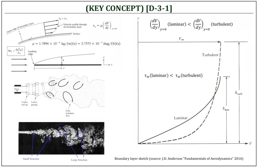
A boundary layer is a thin layer formed on the surface of a solid body in a flow field. Due to the fluid viscosity, the velocity within the boundary layer changes with respect to the vertical distance from the surface. The change of velocity depends on flow field condition, as well as flow type (laminar or turbulent), and usually it is a non-linear change.

The boundary layer “grows” as the flow moves over the surface of a body (the boundary layer “thickness” is defined as: $\delta$ ), and (depending on how the pressure changes in the direction of the flow, i.e., the pressure gradient) may “transition” (from laminar to turbulent) and even “separate” from the surface of a body.

Within the boundary layer, the velocity varies from zero (surface: called the “no-slip” condition) to the free stream (at the edge of the boundary layer): this is called, the “velocity profile” (rate of the shear strain, due to the viscosity) of a boundary layer. At the surface (wall) of a solid body in a viscous flow field, a wall shear stress can be given from fluid mechanics Newtonian fluid viscosity relations, such that:

$\tau_{w} = \mu\left( \frac{dV}{dy} \right)_{y = 0}$

This wall shear stress ( $\tau_{w}$ ) is one of the major contributors to the vehicle drag, called the “skin friction drag.”

A boundary layer, naturally, starts from laminar flow. A laminar boundary layer can be characterized by smooth and regular (predictable) flow field. If visualized, a fluid element moves smoothly along a given streamline in a laminar flow field. Due to multiple contribution factors, a boundary layer transitions from a laminar to a turbulent flow. A turbulent boundary layer can be characterized by random, irregular, and chaotic (not easily predictable) flow field. If visualized, streamlines constantly breakup and a fluid element moves in very unsteady manner. Usually, due to this unsteadiness, turbulent flow field cannot, actually, define any streamline. Transition from laminar to turbulent occurs as Reynolds number of the flow field increases to reach the “transitional Reynolds number” ( ${Re}_{tr}$ ). The actual value of this transitional Reynold number varies depending on the condition of the boundary layer, and usually not easily be predictable.

The shape of the boundary layer also depends on the type of flow (either laminar or turbulent). Usually, a laminar boundary layer is much thicker than a turbulent boundary layer; however, due to a rapid velocity change near the surface of a body for a turbulent flow, the wall shear stress of a turbulent flow tends to be higher than a laminar flow. This leads to the overall higher skin friction drag for a turbulent flow (if compared against a laminar flow). At the same time, a laminar boundary layer (under a rapid increase of pressure in the direction of the flow, i.e., an “adverse pressure gradient” condition) tends to “separate” from the surface of a body (if compared against turbulent boundary layer).

Flat Plate Boundary Layer

Flat Plate Boundary Layer Modeling

KEY CONCEPT [D-3-2]

The analysis of an airfoil’s boundary layer can be done as an extension of the results for a simple flat plate. Effects due to surface curvature and angular acceleration around leading edge can be lumped into a single parameter, the input definition of pressure gradient distribution along the surface. The geometric model is simplified to a flat surface with the pressure gradient and velocity distribution that has been obtained for section inviscid flow analysis.

The height of the boundary layer ( $\delta$ ) can be estimated as the point where $u = 0.99\ U_{\delta}$ . Here $U_{\delta}$ is the velocity of the inviscid flow field outside the viscous boundary layer. In this analysis $U_{\delta}$ is obtained from the previous potential flow panel method solution as the tangential surface velocities on the surface of each of the panels.

Note that the “pressure gradient” along the surface of an airfoil, assuming that pressure is constant in the direction of the depth of the boundary layer, represents the unique 2-D “shape” of the given airfoil, such that:

$\nabla{P} = \frac{\partial P}{\partial x}$

Also, $\tau_{w}$ is the shear stress on the surface (called, the “wall shear stress“) due to friction with the air flow.

The pressure distribution is given by: $P = P_{0} + \frac{1}{2}\rho U_{\delta}^{2}$ for the inviscid external flow, where $P_{0}$ is the stagnation pressure of the flow.

For incompressible flows, the stagnation pressure is constant so that the pressure gradient can be determined as:

$\frac{\partial P}{\partial x} = - \rho U_{\delta}\frac{\partial U_{\delta}}{\partial x}$

The governing equations for this simple one-dimensional flow model can be found by applying the laws of conservation of mass and momentum to a unit depth control volume, covering the boundary layer.

Conservation of mass and momentum ca be defined as:

$\sum_{}^{}{\frac{dm}{dt} = 0\ \ \ \ \text{and}\ \ \ \ \sum_{}^{}{\frac{dm}{dt}u = \sum_{}^{}F_{x}}}$

Mass and Momentum flow will occur at the three free surfaces: inflow side (1), outflow side (2), and (3) edge of the boundary layer ( $v = v_{\delta}$ ), of the given control volume:

$\left( \frac{dm}{dt} \right)_{1} = \int_{0}^{\delta}{\rho u\ dy},\ \ \ \ \left( \frac{dm}{dt} \right)_{2} = - \int_{0}^{\delta}{\left( \rho u + \frac{\partial\rho u}{\partial x}dx \right)dy},\ \ \ \ \text{and}$

$\left( \frac{dm}{dt} \right)_{3} = - \rho v_{\delta}\ dx$

Thus,

$\int_{0}^{\delta}{\frac{\partial\rho u}{\partial x}dxdy} = - \rho v_{\delta}\ dx$

The momentum balance can be determined as:

$\sum_{}^{}{\frac{dm}{dt}u} = - \left( \frac{dm}{dt}u \right)_{1} + \left( \frac{dm}{dt}u \right)_{2} + \left( \frac{dm}{dt}u \right)_{3}$

$= \int_{0}^{\delta}{\left( \rho u^{2} + \frac{\partial\rho u^{2}}{\partial x}dx \right)dy} - \int_{0}^{\delta}{\rho u^{2}\ dy +}\rho U_{\delta}v_{\delta}\ dx$

The horizontal forces on the control volume will come from pressure on inflow side (1) and outflow side (2) and shear stress from the surface:

$\sum_{}^{}F_{x} = P\delta - \left( P + \frac{\partial P}{\partial x} \right)\delta - \tau_{w}dx$

Equating momentum change to applied forces will yield:

$\rho U_{\delta}v_{\delta}dx + \int_{0}^{\delta}{\frac{\partial\rho u^{2}}{\partial x}dxdy} = - \frac{\partial P}{\partial x}\delta_{x} - \tau_{w}dx = \rho U_{\delta}\frac{\partial U_{\delta}}{\partial x} - \tau_{w}dx$

Using the conservation of mass result to substitute for $v_{\delta}$ and cancelling element length $dx$ gives:

$- U_{\delta}\int_{0}^{\delta}{\frac{\partial\rho u}{\partial x}dy} + \int_{0}^{\delta}{\frac{\partial\rho u^{2}}{\partial x}dy} = \rho U_{\delta}\frac{\partial U_{\delta}}{\partial x}\delta - \tau_{w}$

The velocity profile of the layer can be further processed by defining terms specific to its size, displacement effect and momentum loss. Boundary layer thickness ( $\delta$ ) and displacement effect or lost mass flow ( $\delta^{*}$ ) are:

$\delta = \int_{0}^{\delta}{dy}\ \ \ \ \text{and}\ \ \ \ \delta^{*} = \int_{0}^{\delta}{\left( 1 - \frac{\rho u}{\rho_{\delta}U_{\delta}} \right)dy}$

Momentum loss in profile ( $\theta$ ) and wall shear stress ( $\tau_{w}$ ) are:

$\theta = \int_{0}^{\delta}{\frac{\rho u}{\rho_{\delta}U_{\delta}}\left( 1 - \frac{\rho u}{\rho_{\delta}U_{\delta}} \right)dy}\ \ \ \ \text{and}\ \ \ \ \tau_{w} = \left(\mu\frac{\partial u}{\partial y} \right)_{y \rightarrow 0}$

These definitions are applied to low-speed incompressible flow where $\rho$ is constant through the boundary layer ( $\rho_{\delta} = \rho$ ). If the above momentum equation is divided by external momentum, $\rho U_{\delta}^{2}$ , and the above profile definitions are substituted in, then the following form of equation can be obtained:

$\frac{\partial\theta}{\partial x} + \frac{\left( 2\theta + \delta^{*} \right)}{U_{\delta}}\frac{\partial U_{\delta}}{\partial x} - \frac{\tau_{w}}{\rho U_{\delta}} = 0$

For practical purposes, let us define the boundary layer “shape factor, ” such that:

$H = \frac{\delta^{*}}{\theta}$

The value of this boundary layer shape factor does not significantly vary, and this can be used to simplify the solution methods. Therefore:

$\frac{\partial\theta}{\partial x} + (2 + H)\frac{\theta}{U_{\delta}}\frac{\partial U_{\delta}}{\partial x} - \frac{\tau_{w}}{\rho U_{\delta}} = 0$

The solution of this differential equation can be found by starting with initial conditions at the stagnation point, and then integrating along the surface in small steps ( $dx$ ) to find the momentum loss at any point. To simplify calculations, curvature of the airfoil surface is ignored (flat plate), and approximation of polynomial shapes for the boundary layer profile are used to predict local expressions for $\delta$ , $\delta^{*}$ , $\theta$ , and $\tau_{w}$ .

Laminar Flat Plate Boundary Layer

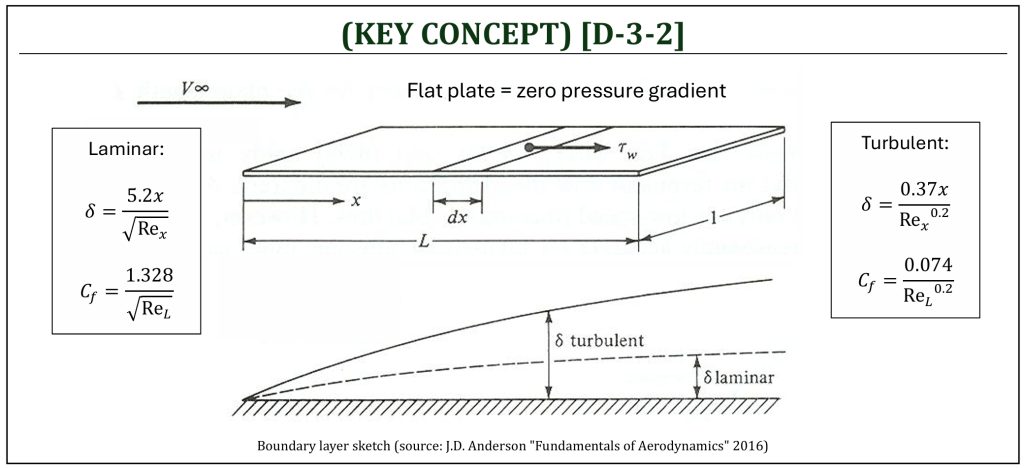
The solution known as “Blasius” solution of flat plate laminar boundary layer (flat plate means “zero pressure gradient“) is given by:

$c_{fx} \equiv \frac{\tau_{w}}{0.5\rho_{\infty}V_{\infty}^{2}} = \frac{\tau_{w}}{q_{\infty}} = \frac{0.664}{\sqrt{{Re}_{x}}}$

Note that the lower case ( $c_{fx}$ ) represents the skin friction drag coefficient “per unit span” at a location $x$ . The skin friction coefficient, due to the wall share stress, will cause the total skin friction drag for the entire flat plate of length $L$ , such that:

$D_{f} = \int_{0}^{L}{\tau_{w}\ dx} = 0.664\ q_{\infty}\int_{0}^{L}\frac{dx}{\sqrt{{Re}_{x}}} = \frac{0.664\ q_{\infty}}{\sqrt{\frac{\rho_{\infty}V_{\infty}}{\mu_{\infty}}}}\int_{0}^{L}\frac{dx}{\sqrt{x}} = \frac{1.328\ q_{\infty}\sqrt{L}}{\sqrt{\frac{\rho_{\infty}V_{\infty}}{\mu_{\infty}}}}$

Then, the total skin friction drag coefficient of the flat plate of length $L$ can be defined as:

$C_{f} \equiv \frac{D_{f}}{q_{\infty}S} = \frac{D_{f}}{q_{\infty}L(1)} = \frac{1.328\ q_{\infty}\sqrt{L}}{q_{\infty}L\sqrt{\frac{\rho_{\infty}V_{\infty}}{\mu_{\infty}}}} = \frac{1.328}{\sqrt{\frac{\rho_{\infty}V_{\infty}L}{\mu_{\infty}}}} = \frac{1.328}{\sqrt{{Re}_{L}}}$

Note that the upper case ( $C_{f}$ ) represents the total skin friction drag coefficient of the given flat plate of length $L$ . In conclusion, for a laminar flat plate boundary layer (Blasius) solution can be applied to predict the boundary layer growth ( $\delta$ ) and the skin friction coefficient ( $C_{f}$ ) for a given flat surface of length $L$ , such that:

$\delta = \frac{5.2 x}{\sqrt{{Re}_{x}}}\ \ \ \ \text{and}\ \ \ \ \ C_{f} = \frac{1.328}{\sqrt{{Re}_{L}}}$

Boundary Layer Transition to Turbulent

Turbulent boundary layer is thicker than the laminar boundary layer, under the same condition of flow. Turbulent boundary layer is often very difficult to analyze and therefore, usually heavily dependent on experimental results. The adverse pressure gradient, rough surface (skin), and many other factors determine boundary layer transition from laminar to turbulent. The physical mechanism of boundary layer transition, even for a simple flat plate, is still not completely understood. The boundary layer transition mechanism is still the area of intensive research in aerodynamics today. Widely accepted empirical turbulent boundary layer solution for a flat plate is given as:

$\delta = \frac{0.37x}{{Re}_{x}^{0.2}}\ \ \ \ \text{and}\ \ \ \ \ C_{f} = \frac{0.074}{{Re}_{L}^{0.2}}$

Laminar and Turbulent Flat Plate Boundary Layer

EXAMPLE [D-3-1]

Flat Plate Boundary Layer with Transition

EXAMPLE [D-3-2]

viscous effects in a flow field

Ideal (potential) v.s. Real Flow Field

KEY CONCEPT [D-3-3]

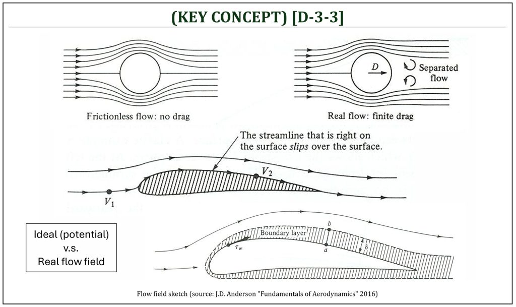
As we learned in potential flow field analysis (B-3 and B-4), the pressure distribution around circular cylinder (ideal flow) is symmetric, thus no lift and no drag will be produced. This is known as d’ Alembert’s paradox. Flow separation, due to the adverse pressure gradient, and resulting complex wake region induces the non-symmetric pressure distribution, thus “pressure drag due to separation” is the main drag contributor of real flows around circular cylinder.

A very similar analogy (that we employed for the analysis of flow over a circular cylinder) can also be applied for the aerodynamics of airfoils and wings. The formation of boundary layer and its behavior (transition from laminar to turbulent flows, as well as the flow separation, due to the pressure gradient) plays very important roles in generations of aerodynamic lift and drag of airfoils and wings.

Let’s understand that the pressure is a function of spatial coordinates. In 2-D Cartesian coordinate system: $p = p(x,y)$ . The mathematical representation of “pressure gradient” ( $\nabla p$ ) is a vector field of the pressure, such that:

Magnitude = maximum rate of change of pressure (per unit length of the coordinate space) at a given point.
Direction = direction of the maximum rate of change of pressure at that given point.

Using this “pressure gradient” representation, directional pressure change in a flow direction ( $s$ ) can be given by:

$\frac{dp}{ds} = \nabla p \cdot \widehat{n}$

This is how much change of pressure takes place in the direction specified by the line vector $\widehat{n}$ : more commonly called physical meaning of the “pressure gradient.” Often, this represents the “airfoil surface shape” itself, as the surface shape directly controls the behavior of the pressure change (either “favorable” or “adverse” change of the pressure on the surface of a body (airfoil).

The pressure gradient along the surface of an airfoil may be favorable (“negative” pressure change) or adverse (“positive” pressure change) in the direction of the given field. Often, an adverse pressure gradient causes flow to be separated from the surface of a body. Flow separation on an airfoil will typically cause:

A sudden and drastic loss of lift (called, the “stall“).
A major increase in drag, caused by pressure drag (called, the “drag due to flow separation“).

At extremely high angles of attack, the flow separates from the top surface of an airfoil, leading it to stall. Desired “post-stall” characteristics (smooth and gradual stall or sudden violent stall) and ease of recovery are important design factors of airfoil (especially important for low-speed and relatively low-altitude operations). It is often important to visualize the surface pressure distributions, as well as the surface streamlines, of a given airfoil under a certain flight condition. If the flow is separated, it will significantly alter the surface pressure distributions. As a result, both “loss of lift” and “increase of drag” will cause the aircraft “stall” condition.

There are two distinctively different types of stall characteristics: “leading edge stall” (for thinner airfoils) and “trailing edge stall” (for thicker airfoils). A thin airfoil (for example: NACA 4412) is desired (typically) for high-speed applications (from high transonic to supersonic) mainly to minimize both “profile” and “wave” drags. However, post-stall behavior is typically associated with “rapid loss” of lift (called, the “leading-edge stall“). this type of behavior is usually not desirable for low-speed operations. A thick airfoil (for example: NACA 4421) is usually desired, especially for low-speed applications (low subsonic), due to the favorable stall characteristics (called, the “trailing-edge stall“).

Skin Friction v.v. Pressure Drag

KEY CONCEPT [D-3-4]

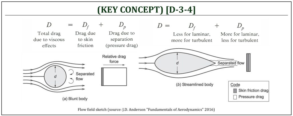
The presence of viscosity in a flow produces two different sources of drag:

Skin friction drag: the drag due to shear stress developed on the surface of the body (called the “wall shear stress“), and this is often called the “parasite drag.”
Pressure drag: the due to flow separation, and this is often called the “drag due to flow separation” (separation drag).

Trade-off between these two drag components may possibly be designed, by carefully engineered pressure coefficient control (i.e., the “shape” of a streamlined body). For example,

Natural Laminar Flow (NLF) airfoil (i.e., NACA 6-series): for more natural laminar flow on the surface of the wing for lower skin friction drag.
Artificial surface roughness control (i.e., dimples of Golf ball): force transition from laminar to turbulent flow for lower pressure drag.

The induced drag ( $C_{D,i}$ ) of a 3-D finite wing is the drag due to lift (3-D effect). The profile drag ( $c_{d}$ ) is a drag on a 2-D airfoil, from which includes: (i) drag due to skin friction (or “parasite“) drag ( $c_{d,f}$ ) and (ii) drag due to pressure (or “separation“) drag ( $c_{d,p}$ ), such that:

$c_{d} = c_{d,f} + c_{d,p}$

In conclusion, the total drag on an aircraft ( $C_{D}$ ) is the sum of profile drag (2-D) and induced drag (3-D) that is:

$C_{D} = c_{d} + C_{D,i} = c_{d,f} + c_{d,p} + \frac{C_{L}^{2}}{\pi eAR}$

References

Fundamentals of Aerodynamics by J.D. Anderson, 5th ED, McGraw Hill, 2016
Aerodynamics for Engineers by J. J. Bertin & M. L. Smith, 3rd ED, Cambridge University Press, 1997
Aerodynamics for Engineering Students by E. L. Houghton & P. W. Carpenter, 4th ED, Edward Arnold, London, 1993

Media Attributions

If a citation and/or attribution to a media (images and/or videos) is not given, then it is originally created for this book by the author, and the media can be assumed to be under CC BY-NC 4.0 (Creative Commons Attribution-NonCommercial 4.0 International) license. Public domain materials have been included in these attributions whenever possible. Every reasonable effort has been made to ensure that the attributions are comprehensive, accurate, and up-to-date. The Copyright Disclaimer under Section 107 of the Copyright Act of 1976 states that allowance is made for purposes such as teaching, scholarship, and research. Fair use is a use permitted by copyright statute. For any request for corrections and/or updates, please contact the author.

License

Icon for the Creative Commons Attribution-NonCommercial 4.0 International License