What is Aerodynamics?

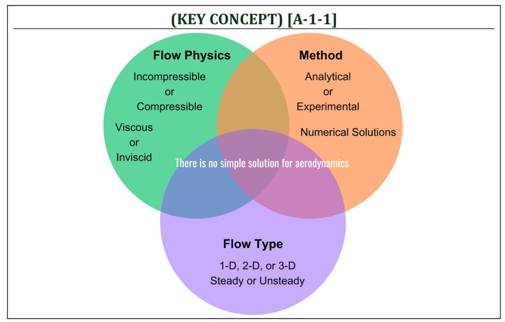
Aerodynamics is a special branch of the broader study area of basic engineering science, that is fluid mechanics.  Therefore, the fundamental masterly understanding of fluid mechanics (i.e., physics of fluid kinematics, statics, and dynamics) is essential to understand aerodynamics.  In order to apply mathematical models to analyze flow field, it is necessary to introduce the following two important constraints in aerodynamics for the purpose of simplification in mathematical analysis:

(i) The first underlying assumption is that the fluid is a continuum (means that the molecular level physics are all intentionally ignored).  This assumption will introduce a hypothetical (non-physical) concept of air particles (i.e., infinitesimally small element of air) that will, as a whole, define a physical flow field to represent the basic physics of a given flow field of air.  In this assumption, many (very many) small (very small) air particles are homogenously distributed throughout a given flow field of air without any chemical component change.  (ii) The second assumption is that the working fluid is a standard air (unlike a liquid, air is an inherently compressible type of fluid and can be modeled by basic gas physics, including the ideal gas law).

Aerodynamics is an incredibly challenging study subject of an extremely wide range of physical variations.  Also, typically the complexity of flow field physics prevents one from fully modeling in a simple mathematical expression.  Simply put, there is no universal mathematical model for the theory of aerodynamics.  Therefore, one needs to carefully approach with multiple physical and mathematical assumptions to simplify a given problem of aerodynamics.  Depending on numbers and types of assumptions, the analysis of aerodynamic modeling can be classified in a few different aerodynamic flow regimes as follows:

Subsonic aerodynamics: is typically, low-speed (Mach number << 1), and main flow field physics will be viscosity modeling (compressibility is usually not a significant contribution factor of flow field physics).  If flow field is assumed to be inviscid (outside of the body surface boundary layer), this is called inviscid low-speed aerodynamics.  If flow field is, further, assumed to be steady (time independent), it is modeled in Euler’s equation as a governing equation for flow field.  If flow field is, further, assumed to be incompressible (Mach number < 0.3), this is incompressible subsonic flow.  It is modeled in Bernoulli’s equation (incompressible form) as a governing equation for flow field.  If flow field is subsonic (Mach number < 1) but compressible ( 0.3 < Mach number), this is compressible subsonic flow.  It is still modeled in energy conservation form of modified Bernoulli’s equation (under the assumption of isentropic flow field).

Transonic aerodynamics: is typically, high subsonic (still Mach number < 1), and compressibility (together with viscosity) can no longer be ignored in flow field physics.  The underlying assumption of continuum with standard air (i.e., ideal gas law) is still applicable, but the flow field physics is quite complicated and mathematical modeling is usually very difficult.

Supersonic aerodynamics: is typically, low supersonic (1 < Mach number < 5), and main flow field physics will be compressibility modeling (viscosity is usually no longer a significant contribution factor of flow field physics).  The underlying assumption of continuum with standard air (i.e., ideal gas law) is still applicable, but usually high-temperature effects (due to energy transfer) in gas physics need to be considered in analysis.

Hypersonic aerodynamics: is typically, high supersonic (5 < Mach number), and the underlying assumption of continuum with standard air (i.e., ideal gas law) can no longer be applicable.  High-temperature effects in gas physics (significant amount of energy transfer analysis with chemical reactions) need to be considered.

Computer Simulation of Aircraft Wing Theory

In order to apply a mathematical scheme for any analysis in aerodynamics, it is crucial to identify assumptions (i.e., constraining conditions or limitations of applicability) of each scheme.  The following list summarizes mathematical methods for analysis in low-speed (subsonic) aerodynamics:

Potential flow analysis: often called ideal flow analysis, with all possible assumptions to simplify flow field physics (i.e., steady, inviscid, incompressible, and irrotational flow field), so that it becomes possible to model flow field in Laplace’s equation as a governing equation.

Conformal mapping analysis: known as Joukowski flow mapping and airfoils that is a simple application of potential flow analysis (a flow over a simple body, such as a circular cylinder, to a flow over a mapped shape of airfoil) in mathematical coordinate transformations.

Panel method analysis: application of potential flow analysis into a 2-D airfoil and/or a 3-D body flow field simulations of any shape (open-source software XFOIL/XFLR5 will be introduced).

Thin airfoil theory analysis: a simplified version of 2-D panel method analysis to compute airfoil characteristics with different cambers (a flat plate with a mean camber line can be analyzed, and thickness of airfoil is ignored).

Lifting Line Theory (LLT) analysis: known as classical Prandtl’s lifting line theory that can model simple 3-D wings without wing sweep (open-source software XFOIL/XFLR5 includes this feature).

Vortex Lattice Method (VLM) analysis: also known as lifting surface method that is an advanced application of Prandtl’s simple lifting line theory to model 3-D wings of any shape (open-source software XFOIL/XFLR5 includes this feature).

Compressibility correction method: known as Prandtl-Glauert correction method to correct analytical results (analytical results are often limited only under incompressible assumption) with compressibility effects (0.3 < Mach number).

Fundamentals of engineering units

It is crucially important for engineers to fully understand and master the usage of proper engineering units.  Many fatal engineering errors are associated with some kind of minor engineering unit mistakes.  In aerodynamics, being a branch of fluid mechanics, we usually employ both SI (International Standard) and US Customary (British Engineering) unit systems under the effects of gravity (this is commonly known as the gravitational unit system).  The standard gravity of earth (at sea-level altitude) can be defined as: 9.81 m/s²  or  32.2 ft/s².

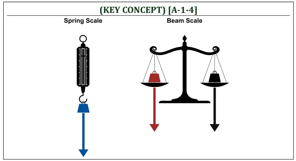
The terms mass and weight are often used almost interchangeably in everyday language.  For example, weight watchers . . . are they trying to control their body mass or body weight (it seems the difference is not so important)?  In aerodynamics (based on physics), however, mass and weight are distinctively different.

First of all . . . what is mass?  Mass is a fundamental property of an object that measures the amount of matters it contains.  Mass is a scalar quantity, meaning it has magnitude but no direction.  Mass is constant over time and does not change with location (this is the principle of conservation of mass).

Then . . . what about weight?  Weight is, in fact, the force of gravity acting on an object’s mass.  Weight varies depending on the strength of the gravitational field.

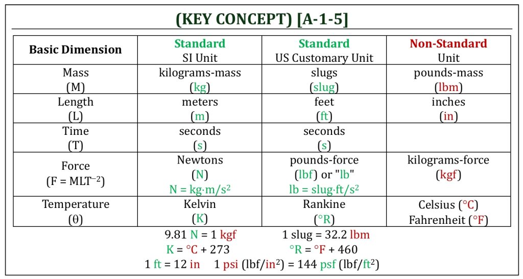
Before casually start using units, one must carefully identify standard (often called as coherent) unit for each engineering entity (i.e., mass (M), length (L), time (T) . . . called basic dimensions of engineering properties).  When, especially, a composite engineering unit (i.e., force (F) is made up by mass, length, and time) is being created, the unit must properly be combined to define appropriate standard composite unit for that property.

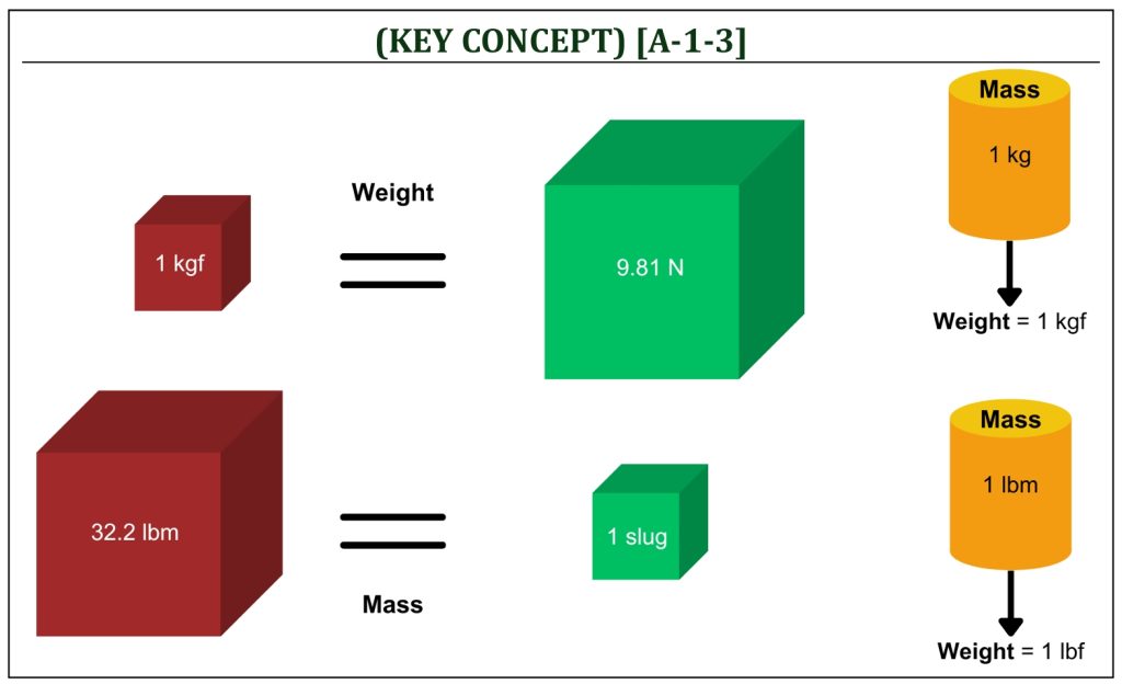
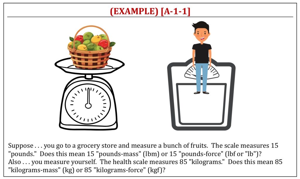
One of the most common mistakes in engineering units is interchangeably using “pounds” (pounds for force or pounds for mass) and/or using “kilograms” (kilograms for mass or kilograms for force).  One is standard (coherent) unit and the other one is not.  If you notice that a non-coherent unit is used, it is required to do the followings:

Non-standard units must always be expressed (always) with subscripts (i.e., lbm for pounds-mass and kgf  for kilograms-force).  If pounds and kilograms are used as standard units (i.e., pounds-force and kilograms-mass), no need to use subscripts (i.e., lb for pounds-force and kg for kilograms-mass).  Often, the standard unit of pounds can be expressed with subscript (i.e., lbf).  While this is acceptable expression to purposefully avoid confusion between lbm and lbf, it is not acceptable to use the standard unit of kilograms with subscript (i.e., kgm), as there is absolutely no such use of unit defined in the SI unit system of kilograms-mass.  Non-standard units (although commonly used) must be unit converted into (less commonly used) standard (coherent) units, i.e., from pounds-mass (lbm) to slugs for mass (US Customary unit system) and from kilograms-force (kgf) to Newtons for force (in SI unit system).  The unit conversions are: 1 slug = 32.2 lbm and 9.81 Newtons = 1 kgf.

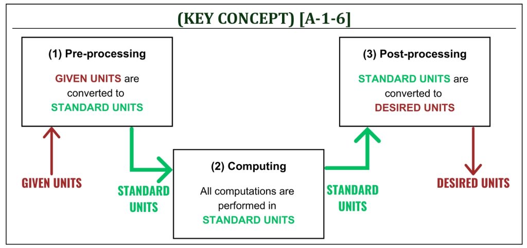
In any engineering analysis, the following 3-stage-analytical-process of unit conversion must be performed as a common practice:

(1) Pre-processing: given units, often non-standard (non-coherent), must be converted into the standard (coherent) unit before computing (computing is usually using your own calculator).
(2) Computing: must be performed with all standard (coherent) units; and therefore, all outputs of computing are all standard (coherent) units.
(3) Post-processing: desired units, often non-standard (non-coherent), must be provided by appropriate unit conversion from outputs of computing.

In aerodynamics, the standard (coherent) units should be employed for flow field properties whenever possible (to minimize any unit mistakes).  Properties of air in a flow field and associated standard units (also associated standard nomenclature) can be summarized below:

Pressure (p) in SI unit is defined as: N/m² (Pascal, or Pa), where: 1,000 Pa = 1 kPa.  Pressure in US Customary unit is defined as: lbf (or lb)/ft² (psf), where commonly used (but not standard unit) is: lbf (or lb)/in² (psi).  Note that the pressure unit conversion can be done by: 1 psi = 144 psf (because 1 ft = 12 inches).

Density (ρ) in SI unit is defined as: kg/m³.  Density in US Customary unit is defined as: slug/ft³, where: 1 slug = 32.2 lbm.

Temperature (T) in SI unit is defined as: Kelvin (K), where K = ºC (Celsius) + 273.  Temperature in US Customary unit is defined as: Rankine (°R), where ºR = °F (Fahrenheit) + 460, where the unit ºR (Rankine) and constant R (specific gas constant of air) should not be confused.

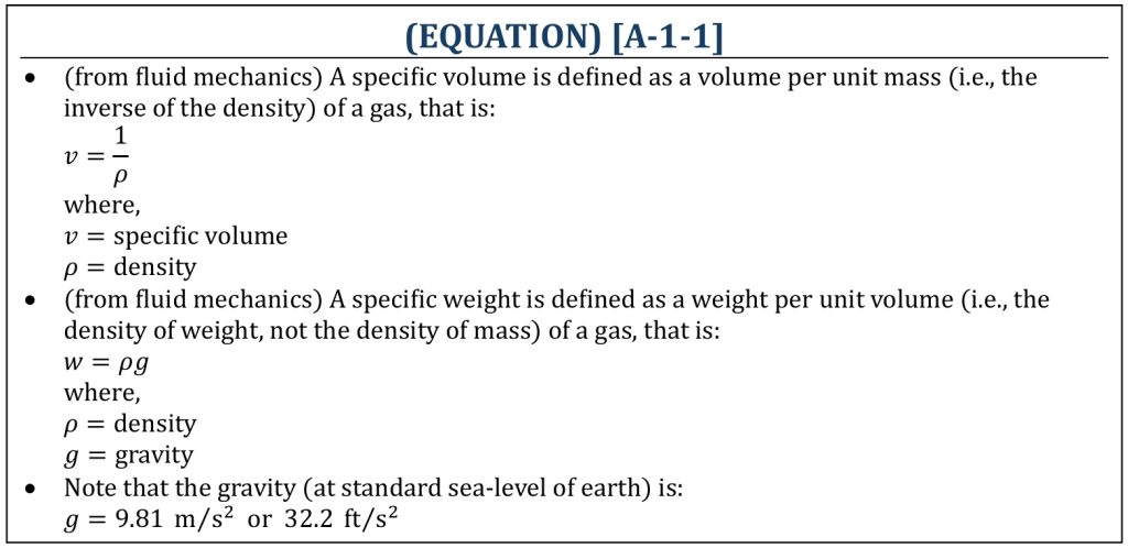
There are a few more additional properties that are important for aerodynamics: a specific volume (v) is an inverse of density (volume per unit mass).  Also, a specific weight (w) is a weight density (weight per unit volume), that can be defined by mass density (ρ) multiplied by gravity (g).  These properties are often confusing and need to be carefully distinguished.

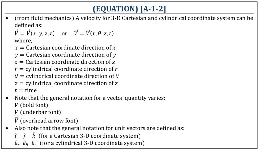
Velocity is a vector property (unlike airspeed that is a scalar), and therefore magnitude and direction must both be specified.  Also, a vector will come with directional components (2 components in 2-D space and 3 components in 3-D space).

There are also a few common mistakes in aerodynamic analysis. One must be extra careful to avoid such mistakes:

• Angle of Attack, or “AOA” (α): may be given in degrees (deg) or radians (rad).  If degrees are used, the equation must include the unit conversion from degrees to radians (180 degrees = π radians).
• Temperature: the problem may be given in relative scales (°C  or °F), but usually need to use absolute scales (K or ºR) in calculations.
• Pressure: you need to know either absolute or gage pressure: i.e., psia or psfa (psi or psf in absolute pressure) or psig or psfg (psi or psf in gage pressure).

Often inches are commonly used, but you should never use inches in your actual calculations: unit conversion will be necessary (1 ft = 12 in) to convert non-standard unit of length (inch) to standard unit of length (feet).  It is never recommended to convert feet (standard unit of length) to inch (non-standard unit of length).

Ideal gas models in aerodynamics

The basic physics of gases (i.e., ideal gas assumption) can certainly be applied to aerodynamics, as long as the flow regime is within reasonable range of Mach number (from subsonic to low-supersonic aerodynamics).  In simple terms, an ideal gas is a theoretical model of gases that helps  to understand and predict how real gases behave.  It is simply a model (not a perfect gas that actually exists in reality) and simplifies the behavior of gases to make calculations and predictions easier.  In aerodynamics, there are two distinctively different models of perfect gases (i.e., ideal gas models) depending on the behavior of the air property, called specific heat.  These are commonly called (i) thermally perfect and (ii) calorically perfect gases.  The distinction between calorically perfect and thermally perfect gases lies in how their specific heats behave with temperature, as follows:

Thermally Perfect Gas: is a gas that adheres to the ideal gas law (called equation of state).  Its internal energy and enthalpy are functions of temperature alone.  However, its specific heats (C_P and Cv) can vary with temperature (details of these different specific heats will be discussed later).  Therefore, these specific heats are not necessarily constant throughout the flow field.  This thermally perfect gas model accounts for the fact that, at higher temperatures, the vibrational energy modes of gas molecules become more significant.  Therefore, higher temperatures tend to increase internal energy and enthalpy much higher rate than lower temperatures.

Calorically Perfect Gas: is a special case of a thermally perfect gas (hence, it also obeys the ideal gas law).  For simplification, its specific heats (C_P and Cv) are assumed to be constant, regardless of temperature.  This simplification is often valid for gases within a moderate temperature range where vibrational energy modes are not significantly excited.  In aerodynamics, this implies typically from subsonic to low-supersonic flow regime without combustion and/or shockwave interactions involved..  The equation of state for an ideal gas can be given below.

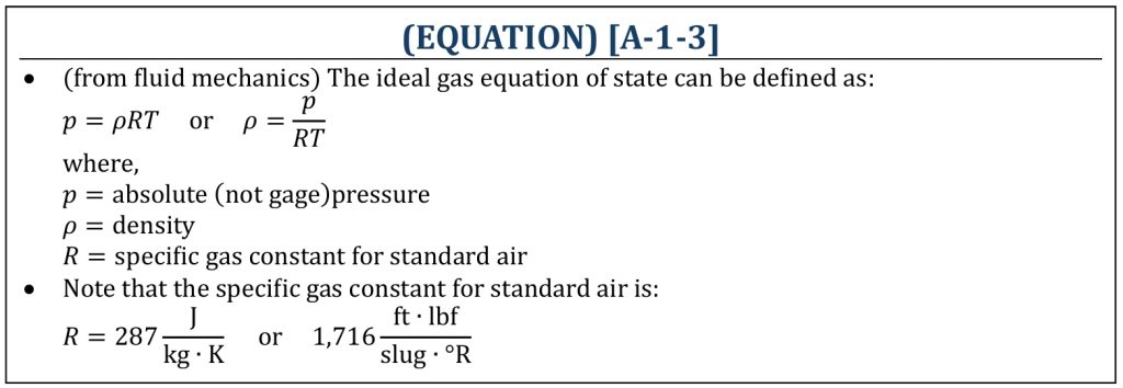
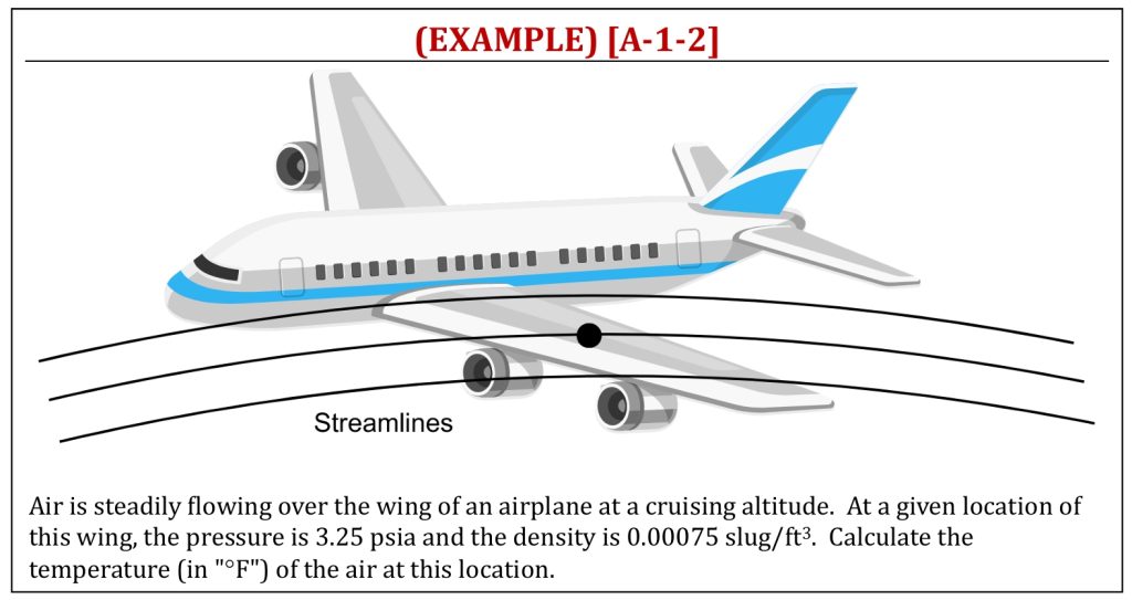
In essence, all calorically perfect gases are thermally perfect, but not all thermally perfect gases are calorically perfect.  The key difference is whether the specific heats are constant (calorically perfect gas) or variable with respect to the temperature (thermally perfect gas).  If it is assumed that the specific heat of air stays the same (i.e., low-speed flows), it can be treated as a calorically perfect gas.  If it is required to account for changes in specific heat due to temperature variations (i.e., high-speed flows), it is required to model as a thermally perfect gas.  For the ideal gas equation of state, pressures must always be in absolute pressures (not gage pressures).  Also, temperatures must always be in absolute scale (K / °R), not in relative scale (°C / °F) temperatures.  For the cases of calorically perfect ideal gases of air, it is also possible to define the gas constant, that is specific to the standard air.

Flow Field Representations and viscous effects

As it was introduced in fluid mechanics, there are two different fundamental modeling approaches to represent flow field physics.  The Lagrangian and the Eulerian approaches are two fundamental ways to describe the motion of a fluid or other continuous medium.  They differ in their frame of reference and resulting mathematical formulations are quite different:

• Lagrangian approach: is a trace of motion of each (and all) individual small particles to represent a flow field. This is inherently a differential type of mathematical analysis and usually produces a governing differential equation to represent a flow field.
• Eulerian approach: is an integration of flow field (often within a limited space in a flow field, called a control volume).  The Reynolds Transport Theorem can be applied for a control volume to integrate governing differential equation to actually solve the problem.  Often, however, some assumptions must be applied to simplify the equation (i.e., steady flow field).

In order to visualize a given flow field, typically the following three different lines can be defined:

• A streakline: is a line defined in a flow field by continuously injecting infinitesimally small particles at a fixed location.  Generating a series of streaklines (i.e., smoke wind tunnel) is essentially a pure experimental method and fundamentally an Eulerian approach.
• A pathline: is a line defined by tracing a path of an individual particle.  A series of pathlines can be visualized by injecting small particles in the flow field and tracing each of them (i.e., Particle Image Velocimetry, or PIV).  Generating a series of pathlines involves a large number of particle traces with full description of motion (i.e., equation of motion for each particle) and fundamentally a Langrangian approach.  Needless to say, this is usually extremely resource intensive and may not be able to fully represent the entire flow field.
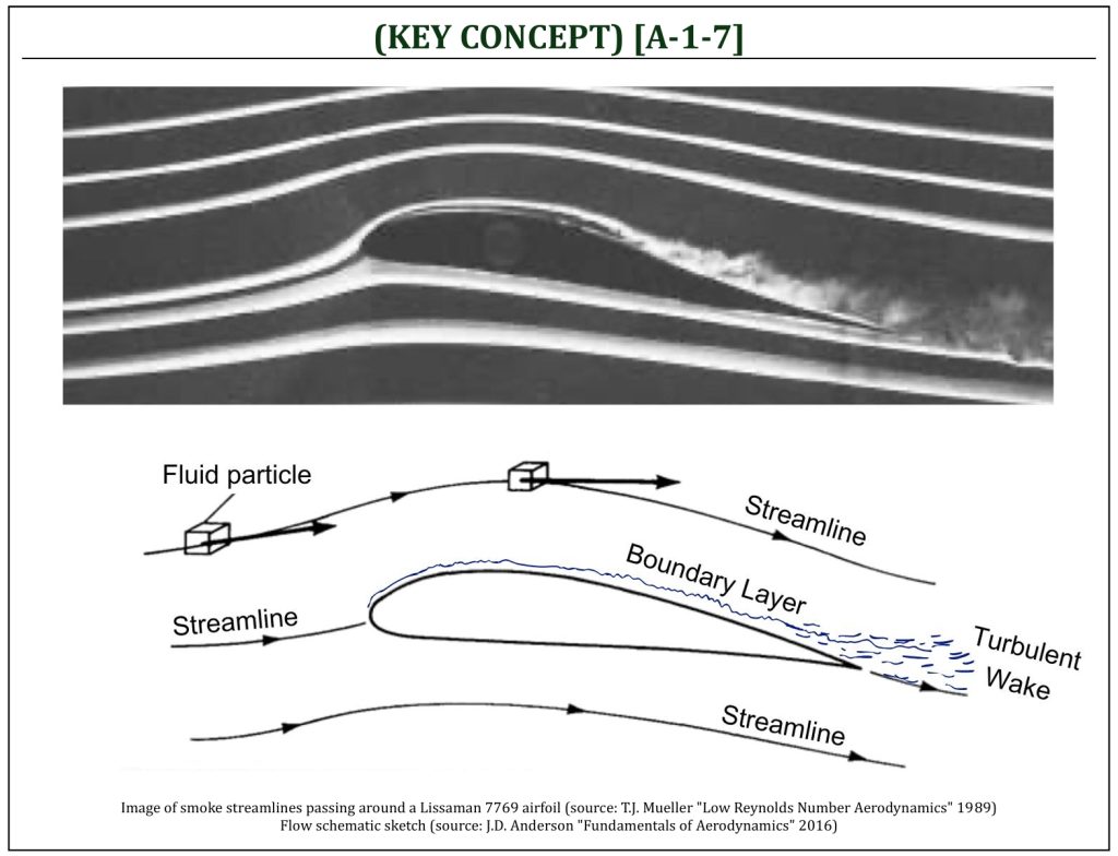
• A streamline: for a steady flow field, a moving fluid element traces out a fixed path in space.  This can be represented by a streamline.  The streamline is a mathematical concept (can be represented by stream functions and equations of streamlines).  In terms of flow field physics, a streamline is a line at which the velocity (at each location along the line) is tangent along its path.  As a matter of fact, a stream function is a mathematical solution of a potential (often called an ideal) flow field that is governed by the Laplace’s equation.  Mathematically solving a potential flow field is a fundamental scheme for the theory of aerodynamics (this will be discussed later in more details).

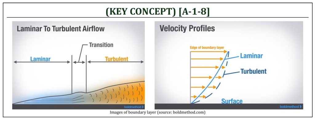
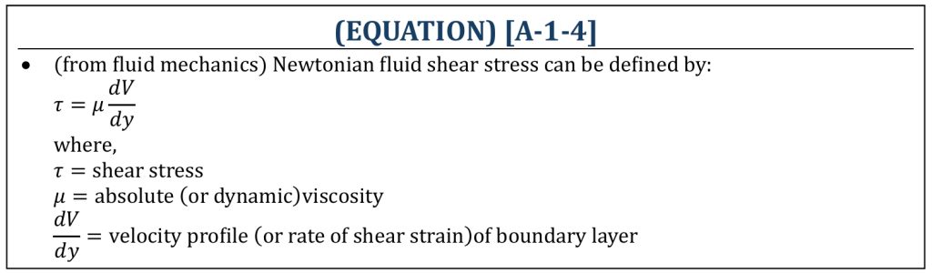
In aerodynamics, often the effects of viscosity will be separately analyzed (inviscid external flow outside of the body surface boundary layer and viscous internal flow within the boundary layer).  External flow field (outside of boundary layer) can be analyzed by application of Euler’s equation.  If viscosity is included, the shear stress due to viscosity (within the boundary layer) must also be included in the analysis.  From fluid mechanics, simple Newtonian shear stress model will be employed for viscous flow field (i.e., boundary layer analysis).

References

• Xflr5 by techwinder (www.xflr5.tech/xflr5.htm)
• BoldMethod (www.boldmethod.com)
• Fundamentals of Aerodynamics by J.D. Anderson, 5th ED, McGraw Hill, 2016
• Aerodynamics for Engineers by J. J. Bertin & M. L. Smith, 3rd ED, Cambridge University Press, 1997
• Aerodynamics for Engineering Students by E. L. Houghton & P. W. Carpenter, 4th ED, Edward Arnold, London, 1993
• Low Reynolds Number Aerodynamics by T.J. Mueller, 1989

Media Attributions

If a citation and/or attribution to a media (images and/or videos) is not given, then it is originally created for this book by the author, and the media can be assumed to be under CC BY-NC 4.0 (Creative Commons Attribution-NonCommercial 4.0 International) license.  Public domain materials have been included in these attributions whenever possible.  Every reasonable effort has been made to ensure that the attributions are comprehensive, accurate, and up-to-date. The Copyright Disclaimer under Section 107 of the Copyright Act of 1976 states that allowance is made for purposes such as teaching, scholarship, and research.  Fair use is a use permitted by copyright statute.  For any request for corrections and/or updates, please contact the author.