What is real-time PCR?

The polymerase chain reaction (PCR) is one of the most powerful technologies in molecular biology. Using PCR, specific sequences within a DNA or cDNA template can be copied, or “amplified”, many thousand- to a million-fold using sequence-specific oligonucleotides, heat-stable DNA polymerase, and thermal cycling. In traditional endpoint PCR, detection and quantification of the amplified sequence are performed at the end of the reaction after the last PCR cycle, and involve post-PCR analysis such as gel electrophoresis and image analysis. In real-time quantitative PCR (qPCR, RT-qPCR), the concentration of the PCR products is measured after each cycle. By monitoring reactions during the exponential amplification phase of the reaction, we can determine the initial quantity of the target with great precision. PCR theoretically amplifies DNA exponentially, doubling the number of target molecules with each amplification cycle. In this technique, the amount of DNA is measured using fluorescent dyes that yield an increasing fluorescent signal in direct proportion to the number of PCR product molecules (amplicons) generated, providing information on the starting quantity of the amplification target. Fluorescent reporters used in real time PCR include double-stranded DNA (dsDNA)–binding dyes, or dye molecules attached to PCR primers or probes that hybridize with PCR products during amplification. The change in fluorescence over the course of the reaction is measured by an instrument that combines thermal cycling with fluorescent dye scanning capability. By plotting fluorescence against the cycle number, the real-time PCR instrument generates an amplification plot that represents the accumulation of product over the duration of the entire PCR reaction.

Real-time PCR steps

If a particular sequence (DNA orRNA) is abundant in the sample, amplification is observed in earlier cycles; if the sequence is scarce, amplification is observed in later cycles.

Denaturation: High-temperature incubation is used to “melt” double-stranded DNA into single strands and loosen secondary structure in single-stranded DNA. The highest temperature that the DNA polymerase can withstand is typically used (usually 95 C). The denaturation time can be increased if the template GC content is high.

Annealing: During annealing, complementary sequences have an opportunity to hybridize, so an appropriate temperature is used that is based on the calculated melting temperature (Tm) of the primers (typically 5 C below the Tm of the primer).

Extension: At 70–72 C, the activity of the DNA polymerase is optimal, and primer extension occurs at rates of up to 100 bases per second. When an amplicon in real-time PCR is small, this step is often combined with the annealing step, using 60 C as the temperature.

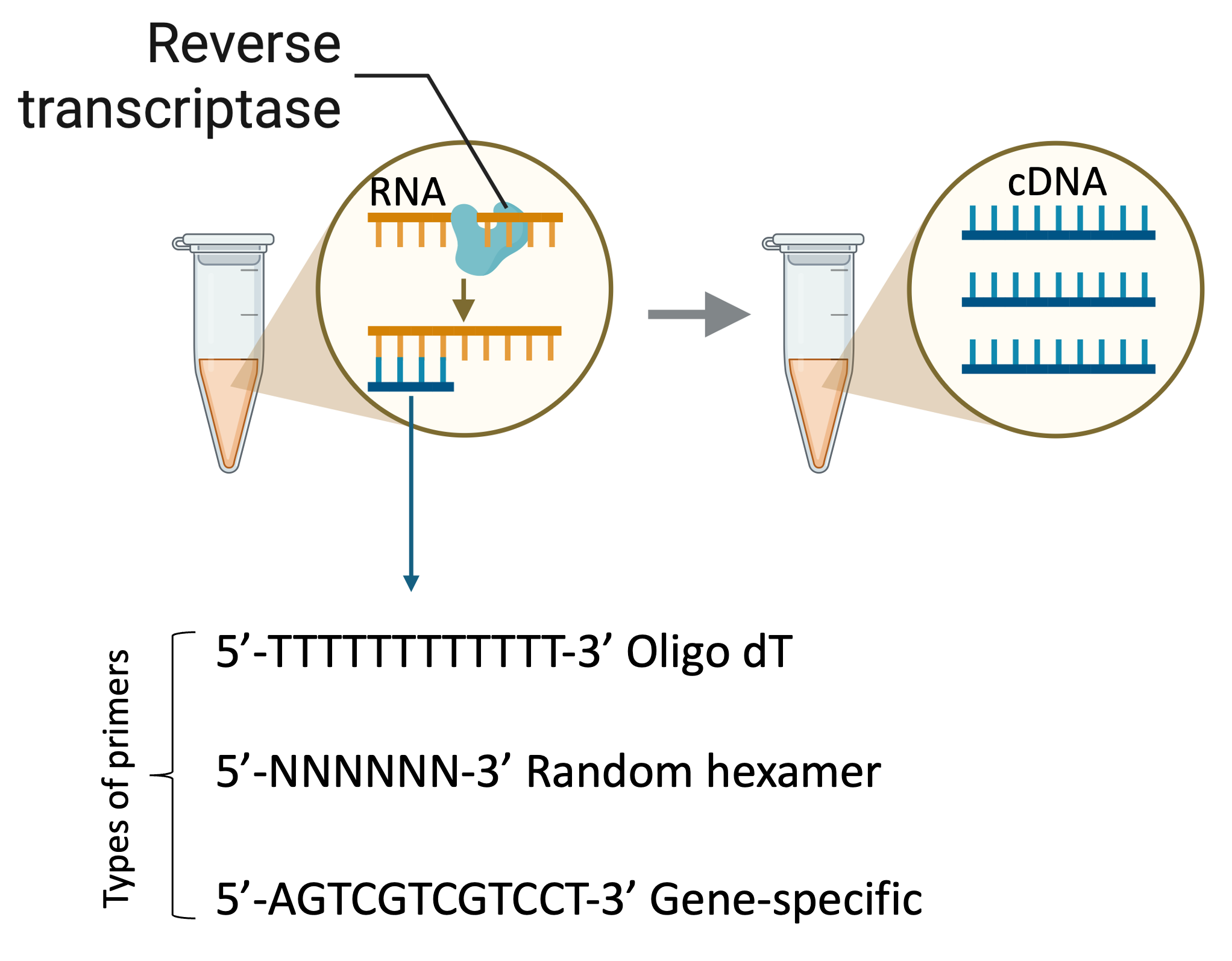
Two-step RT-qPCR

Two-step quantitative reverse transcriptase PCR (RT-qPCR) starts with the reverse transcription of either total RNA or poly(A) RNA into cDNA using a reverse transcriptase (RT). This first-strand cDNA synthesis reaction can be primed using random, oligo(dT), or gene-specific primers. The temperature used for cDNA synthesis depends on the RT enzyme chosen, generally between 40-45 C. After reverse transcription an aliquot of the cDNA is transferred to a separate tube for the real-time PCR reaction.

One-step RT-qPCR

One-step RT-qPCR combines the first-strand cDNA synthesis reaction and real-time PCR reaction in the same tube, simplifying reaction setup and reducing the possibility of contamination. Gene-specific primers (GSP) are required because using oligo(dT) or random primers will generate nonspecific products in the one-step procedure and reduce the amount of product of interest.

Real-time PCR analysis

Baseline

The baseline of the real-time PCR reaction refers to the signal level during the initial cycles of PCR, usually cycles 3 to 15, in which there is little change in fluorescent signal. The low-level signal of the baseline can be equated to the background or the “noise” of the reaction. The baseline in real-time PCR is determined empirically for each reaction, by user analysis or automated analysis of the amplification plot. The baseline should be set carefully to allow accurate determination of the threshold cycle (Ct), defined below. The baseline determination should consider enough cycles to eliminate the background found in the early cycles of amplification, but should not include the cycles in which the amplification signal begins to rise above background. When comparing different real-time PCR reactions or experiments, the baseline should be defined in the same way for each.

Threshold

The threshold of the real-time PCR reaction is the level of signal that reflects a statistically significant increase over the calculated baseline signal. It is set to distinguish relevant amplification signal from the background. Usually, real-time PCR instrument software automatically sets the threshold at 10 times the standard deviation of the fluorescence value of the baseline.

Ct (threshold cycle)

The threshold cycle (Ct) is the cycle number at which the fluorescent signal of the reaction crosses the threshold. The Ct is used to calculate the initial DNA copy number, because the Ct value is inversely related to the starting amount of target. For example, in comparing real-time PCR results from samples containing different amounts of target, a sample with twice the starting amount will yield a Ct one cycle earlier than a sample with twice the number of copies of the target, relative to a second sample, will have a Ct one cycle earlier than that of the second sample. This assumes that the PCR is operating at 100% efficiency (i.e., the amount of product doubles perfectly during each cycle) in both reactions. As the template amount decreases, the cycle number at which significant amplification is seen, increases too. With a 10-fold dilution series, the Ct values are ~3.3 cycles apart.

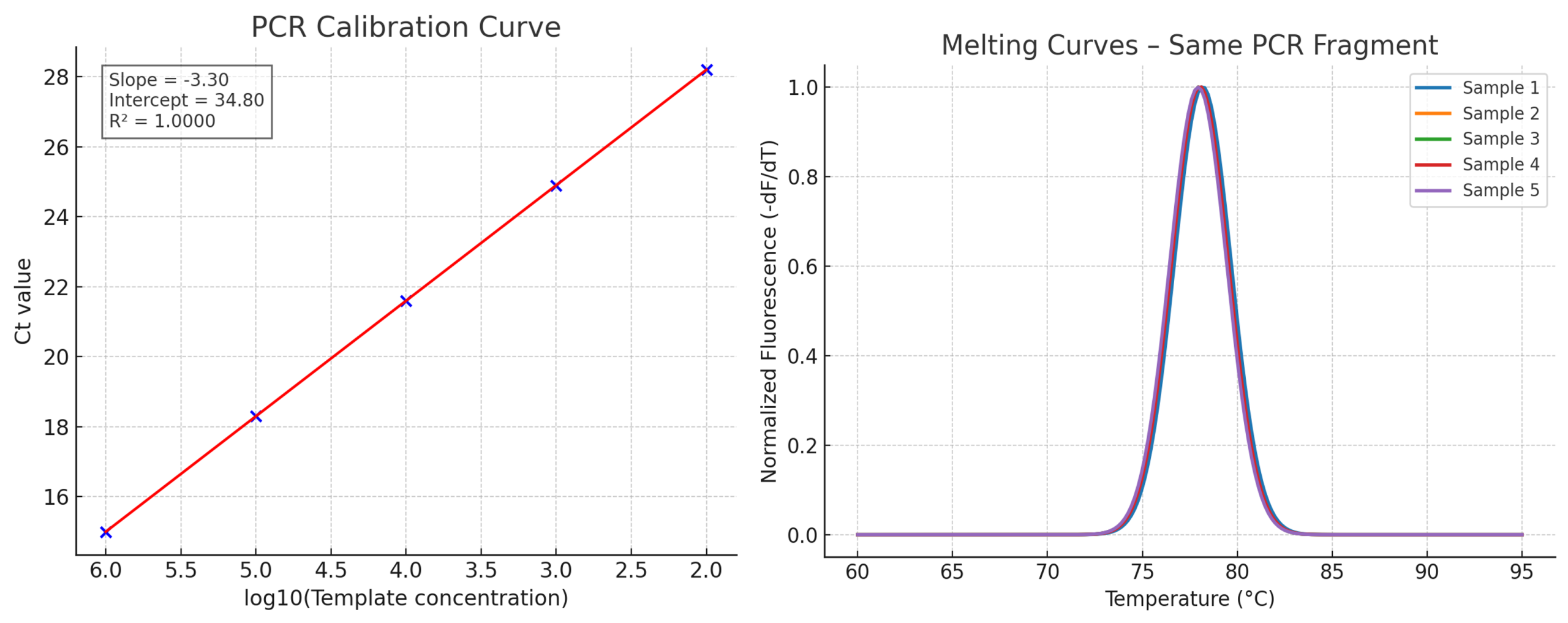
Standard curve

A dilution series of known template concentrations can be used to establish a standard curve to determine the initial starting amount of the target template in experimental samples or to assess the reaction efficiency. The log of each known concentration in the dilution series (x-axis) is plotted against the Ct value for that concentration (y-axis). From this standard curve, information about the performance of the reaction as well as various reaction parameters (including slope, y-intercept, and correlation coefficient) can be derived. The concentrations chosen for the standard curve should encompass the expected concentration range of the target in the experimental samples.

Correlation coefficient (R2)

The correlation coefficient is a measure of how well the data fit the standard curve. The R2 value reflects the linearity of the standard curve. Ideally, R2 = 1, although 0.999 is generally the maximum value. 

Y-intercept

The y-intercept corresponds to the theoretical limit of detection of the reaction, or the Ct value expected if the lowest copy number of target molecules denoted on the x-axis gave rise to statistically significant amplification. Though PCR is theoretically capable of detecting a single copy of a target, a copy number of 2–10 is commonly specified as the lowest target level that can be reliably quantified in real-time PCR applications. This limits the usefulness of the y-intercept value as a direct measure of sensitivity. However, the y-intercept value may be useful for comparing different amplification systems and targets.

Exponential phase

It is important to quantify your real-time PCR reaction in the early part of the exponential phase as opposed to in the later cycles or when the reaction reaches the plateau. At the beginning of the exponential phase, all reagents are still in excess, the DNA polymerase is still highly efficient, and the amplification product, which is present in a low amount, will not compete with the primers’ annealing capabilities. All of these factors contribute to more accurate data.

Slope

The slope of the log-linear phase of the amplification reaction is a measure of reaction efficiency. To obtain accurate and reproducible results, reactions should have an efficiency as close to 100% as possible, equivalent to a slope of –3.32.

Amplification efficiency

A PCR efficiency of 100% corresponds to a slope of –3.32, as determined by the following equation:

                                            Efficiency = 10^(–1/slope)

Ideally, the efficiency (E) of a PCR reaction should be 100%, meaning the template doubles after each thermal cycle during exponential amplification. The actual efficiency can give valuable information about the reaction. Experimental factors such as the length, secondary structure, and GC content of the amplicon can influence efficiency. Other conditions that may influence efficiency are the dynamics of the reaction itself, the use of non-optimal reagent concentrations, and enzyme quality, which can result in efficiencies below 90%. The presence of PCR inhibitors in one or more of the reagents can produce efficiencies of greater than 110%. A good reaction should have an efficiency between 90% and 110%, which corresponds to a

slope of between –3.58 and –3.10.

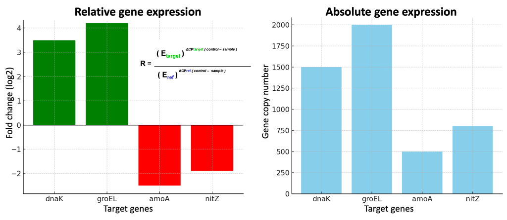
Absolute quantification

Absolute quantification describes a real-time PCR experiment in which samples of known quantity are serially diluted and then amplified to generate a standard curve. Unknown samples are then quantified by comparison with this curve.

Relative quantification

Relative quantification describes a real-time PCR experiment in which the expression of a gene of interest in one sample (i.e., treated) is compared to expression of the same gene in another sample (i.e., untreated). The results are expressed as fold change (increase or decrease) in expression of the treated sample in relation to the untreated sample. A reference gene (such as β-actin) is used as a control for experimental variability in this type of quantification.

Melting curve (dissociation curve)

A melting curve shows the change in fluorescence observed when double-stranded DNA (dsDNA) with incorporated dye molecules dissociates (“melts”) into single-stranded DNA (ssDNA) as the temperature of the reaction is raised. For example, when double-stranded DNA bound with SYBR Green I dye is heated, a sudden decrease in fluorescence is detected when the melting point (Tm) is reached, due to dissociation of the DNA strands and subsequent release of the dye. The fluorescence is plotted against temperature, and then the –ΔF/ΔT (change in fluorescence/ change in temperature) is plotted against temperature to obtain a clear view of the melting dynamics.

Post-amplification melting-curve analysis is a simple, straightforward way to check real-time PCR reactions for primer-dimer artifacts and to ensure reaction specificity. Because the melting temperature of nucleic acids is affected by length, GC content, and the presence of base mismatches, among other factors, different PCR products can often be distinguished by their melting characteristics. The characterization of reaction products (e.g., primer dimers vs. amplicons) via melting curve analysis reduces the need for time-consuming gel electrophoresis.

Adapted from Life Technologies Real-time PCR Handbook.

Materials

Micropipette set

Micropipette tips

Microcentrifuge

Microcentrifuge tubes

PCR plates

Real-time thermocycler

cDNA template (from your last experiment)

RT PCR mastermix reagents

Safety concerns

This PCR experiment uses chemicals, biological materials, and equipment  that pose some potential risks:

1. Handle the reagents with gloves, at all times.
2. Use biosafety protocols to handle the DNA samples  to prevent accidental exposure, and dispose of all the waste in a biohazard container.
3. Make sure you balance the microcentrifuges correctly before you use them.
4. Avoid eating or drinking, and manage spills and emergencies following the directions of the instructor.

Reverse transcription (qMax First strand cDNA synthesis Flex kit)

1. Thaw template RNA and all reagents on ice. Mix each solution by vortexing, and centrifuge briefly to collect residual liquid from the sides of the tubes.
2. Prepare the following mastermix in a PCR tube on ice:

3. Incubate at 25 C for 10 min if a random primer is used.
4. Incubate the mixture at 42 C for 60 min.
5. Stop the reaction by heating the samples at 70 C for 10 min.
6. Chill samples on ice. The newly synthesized first-strand cDNA now can be used directly for PCR amplification or it can be stored at -20 C.

Real-time PCR (qMax Green Low ROX qPCR Mix)

1. Mix the components thoroughly, except for the cDNA template, then spin down the contents and eliminate any air bubbles.

2. Transfer 16 uL of mastermix to each of 3 wells of an optical plate.
3. Add the cDNA template on the corresponding wells or water in the negative control.
4. Seal the plate with an optical adhesive cover, then centrifuge briefly to spin down the contents and eliminate any air bubbles.
5. Place the reaction plate in the real-time PCR instrument.
6. Set the thermal cycling conditions using the default PCR thermal cycling conditions specified in the following tables according to the instrument cycling parameters and melting temperatures of the specific primers.
7. At the end of the program, include an additional one to create a dissociation curve.

Analysis

7. View the amplification plots.
8. Calculate the baseline and threshold cycles (CT) for the amplification curves using the instrument software.
9. Check for nonspecific amplification using dissociation curves.
10. Perform relative quantitation.

Differential gene expression estimation using the Pfaffl equation

1. Calculate the primers amplification efficiencies. In other words, calculate the actual increase in the number of amplicons on each of your reactions after each amplification cycle. This has been calculated for you by your instructor and the number for all genes is 2.
2. Average the technical replicates for all genes and treatments. For each gene of interest (GOI) and reference gene you must have 4 values: GOI treatment, GOI control, REF treatment, REF control.
3. Calculate the Delta-Ct values by subtracting the average treatment Ct from the average control Ct for each GOI and REF.
4. Enter the values into the Pfaffl equation:

5. Transform the ratios (R ) to log2 so instead of fractions you obtain negative values.
6. Create a bar graph showing the log2 values for each of the GOI’s.