C-4: Panel Methods

Shigeo Hayashibara

C-4: Panel Methods

2-D Source Panel Method and Vortex Panel Method

Shigeo Hayashibara

2-D Source Panel Method

Source Panel

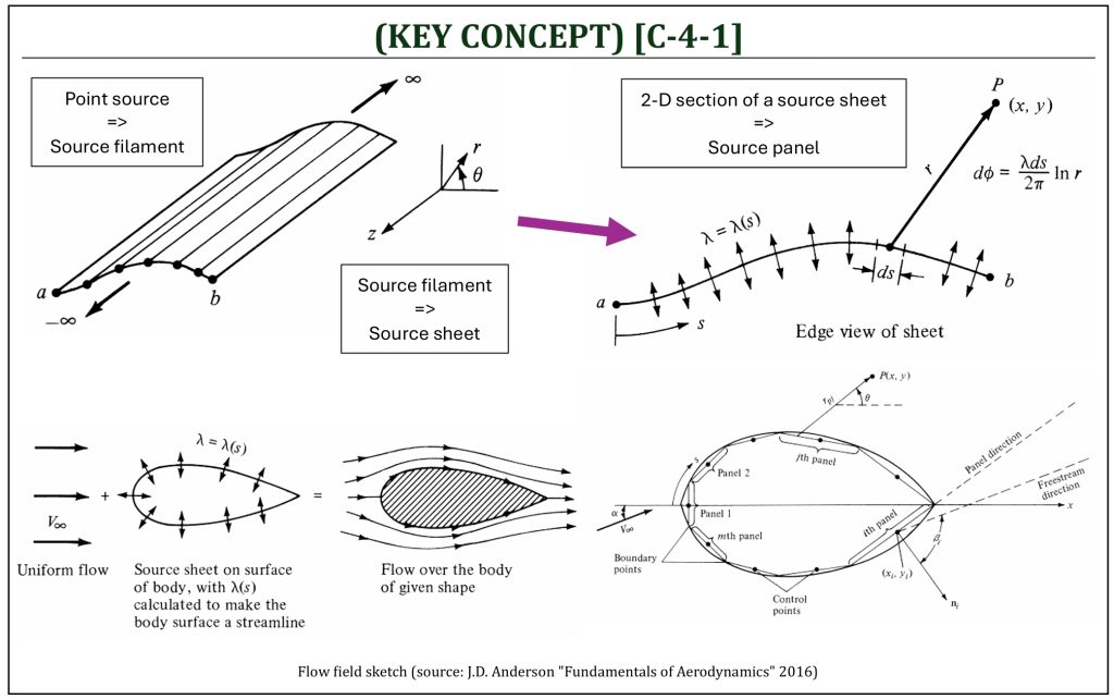
Similar to a vortex panel (discussed in C-3), a source sheet can be defined as infinite number of line sources (side by side) where the strength of each line source is infinitesimally small. Source strength per unit length can be defined by $\lambda = \lambda(s)$ .

Consider an arbitrary point: $P(x,y)$ . A small section of the source sheet of strength ( $\lambda ds$ ) induces an infinitesimally small velocity potential $d\phi$ :

$d\phi = \frac{\lambda ds}{2\pi}\ln(r)$

Thus, the complete velocity potential at point $P$ induced by the entire source sheet can be determined, such that:

$\phi(x,y) = \int_{a}^{b}{\frac{\lambda ds}{2\pi}\ln(r)}$

Let us approximate the source sheet by a series of straight source panels; moreover, let the source strength per unit length be constant over a given panel. For the total number of $n$ panels, the source strengths per unit length for each panel can be represented by:

$\lambda_{1},\ \lambda_{2},\ \lambda_{3},\ .\ \ .\ \ .\ ,\lambda_{j},\ .\ \ .\ \ .\ ,\lambda_{i},\ .\ \ .\ \ .\ ,\lambda_{n}$

Then, it is solved that: $\lambda_{j},\ j = 1,\ 2,\ 3,\ \ \ .\ \ .\ \ .\, n$ such that the body surface becomes a streamline of the flow. It means that the boundary condition is imposed numerically for each of $\lambda_{j}$ , such that the normal component of the flow velocity is zero at the midpoint (called, the “control point“) of each source panel.

Again, consider a point $P(x,y)$ in the flow field, and let $r_{pj}$ be the distance from any point on the $j$ th panel to $P$ . The velocity potential induced at $P$ due to the $j$ th panel is:

$\Delta\phi_{j} = \frac{\lambda_{j}}{2\pi}\int_{j}^{\ }{\ln{\left( r_{pj} \right)ds_{j}}}$

The potential at $P$ due to all panels is, therefore:

$\phi(P) = \sum_{j = 1}^{n}{\Delta\phi_{j}} = \sum_{j = 1}^{n}{\frac{\lambda_{j}}{2\pi}\int_{j}^{\ }{\ln{\left( r_{pj} \right)ds_{j}}}}$

where,

$r_{pj} = \sqrt{\left( x - x_{j} \right)^{2} + \left( y - y_{j} \right)^{2}}$

Next, let us place $P$ at the control point of the $i$ th panel, that is: $P\left(x_{i}, y_{i}\right)$ :

$\phi\left( x_{i},\ y_{i} \right) = \sum_{j = 1}^{n}{\frac{\lambda_{j}}{2\pi}\int_{j}^{\ }{\ln{\left( r_{ij} \right)ds_{j}}}}$

where,

$r_{ij} = \sqrt{\left( x_{i} - x_{j} \right)^{2} + \left( y_{i} - y_{j} \right)^{2}}$

This is the velocity potential (the contribution of all panels to the potential at the control point of the $i$ th panel). Next, the freestream component normal to the panel can be determined as:

$V_{\infty,n} = {\overrightarrow{V}}_{\infty} \cdot {\widehat{n}}_{i} = V_{\infty}\cos\left\lbrack \beta_{i} \right\rbrack$

The normal component of the velocity induced at the control point ( $x_{i}, y_{i}$ ) by a panel is:

$V_{n} = \frac{\partial}{\partial n_{i}}\left\lbrack \phi\left(x_{i}, y_{i}\right)\right\rbrack$

$= \frac{\partial}{\partial n_{i}}\left\lbrack \sum_{j = 1}^{n}{\frac{\lambda_{j}}{2\pi}\int_{j}^{\ }{\ln{\left( r_{ij} \right)ds_{j}}}} \right\rbrack$

$= \frac{\lambda_{i}}{2} + \sum_{j = 1}^{n}{\frac{\lambda_{j}}{2\pi}\int_{j}^{\ }{{\frac{\partial}{\partial n_{i}}\ln}{\left( r_{ij} \right)ds_{j}}}}$

Then, applying the boundary condition ( $V_{\infty,n} + V_{n} = 0$ ) with simplification of:

$I_{i,j} = \int_{j}^{\ }{{\frac{\partial}{\partial n_{i}}\ln}{\left( r_{ij} \right)ds_{j}}}$

In conclusion, the governing equation of 2-D source panel method is constructed, as:

$\frac{\lambda_{i}}{2} + \sum_{j = 1}^{n}\frac{\lambda_{j}}{2\pi}I_{i,j} + V_{\infty}\cos\left\lbrack \beta_{i} \right\rbrack = 0$

This is a series of linear algebraic equation with $n$ unknowns:

$\lambda_{1},\ \lambda_{2},\ \lambda_{3},\ .\ \ .\ \ .\ ,\lambda_{j},\ .\ \ .\ \ .\ ,\lambda_{i},\ .\ \ .\ \ .\ ,\lambda_{n}$

and these unknowns can be solved ( $n$ equations with $n$ unknowns (requires a matrix solver). Once all unknown $\lambda$ are solved ( $\lambda_{1},\ \lambda_{2},\ \lambda_{3},\ .\ \ .\ \ .\ ,\lambda_{j},\ .\ \ .\ \ .\ ,\lambda_{i},\ .\ \ .\ \ .\ ,\lambda_{n}$ ), then the surface velocity of each panel (at each control point) can be determined. The component of freestream velocity tangent to the surface (called, the “tangential” velocity) is, then:

$V_{\infty,s} = V_{\infty}\sin\left( \beta_{i} \right)$

The tangential velocity ( $V_{s}$ ) at the control point of the $i$ th panel, induced by all the source panels is:

$V_{s} = \frac{\partial\phi}{\partial s} = \sum_{j = 1}^{n}\frac{\lambda_{i}}{2\pi}\int_{j}^{\ }{\frac{\partial}{\partial s}\left\lbrack \ln\left( r_{ij} \right) \right\rbrack ds_{j}}$

The total surface velocity at the $i$ th control point ( $V_{i}$ ) is the sum of the contribution from the freestream and from the source panels, hence:

$V_{i} = V_{\infty,s} + V_{s} = V_{\infty}\sin{\left( \beta_{i} \right) + \sum_{j = 1}^{n}\frac{\lambda_{i}}{2\pi}\int_{j}^{\ }{\frac{\partial}{\partial s}\left\lbrack \ln\left( r_{ij} \right) \right\rbrack ds_{j}}}$

Finally, the pressure coefficient at the $i$ th panel can be calculated by:

${Cp}_{i} = 1 - \left( \frac{V_{i}}{V_{\infty}} \right)^{2}$

2-D Vortex Panel Method

At this moment, let us review KEY CONCEPT [C-3-1] once again. As discussed in C-3, (thin airfoil theory), a vortex filament can be defined as a straight line, made by a series of point vortices, going through point O (extended to infinity on both sides). A vortex “sheet” (or “panel” in 2-D cross section) can be defined as infinite number of vortex filaments side by side, with the strength of each filament is infinitesimally small. Once again, considering an arbitrary point $P(x,y)$ , a small section of vortex sheet of strength ( $\gamma ds$ ) induces a small velocity potential ( $d\phi$ ) and velocity ( $dV$ ):

$d\phi = - \frac{\gamma ds}{2\pi}\theta\ \ \ \ \text{and}\ \ \ \ \ dV = - \frac{\gamma ds}{2\pi r}$

The velocity potential at location $P(x,z)$ due to entire vortex sheet from location $a$ to location $b$ can be calculated, such that:

$\phi(x,z) = - \frac{1}{2\pi}\int_{a}^{b}{\theta\ \gamma ds}$

where,

$\int_{a}^{b}{\ \gamma ds} = \Gamma\ (\text{circulation})$

An very similar approach (as discussed in source panel method) can be taken again for vortex panel method. A series of vortex sheets approximates the body of arbitrary shape (vortex panels). The total number of $n$ panels are defined with the vortex strengths per unit length ( $\gamma = \gamma(s)$ ) of:

$\gamma_{1},\ \gamma_{2},\ \gamma_{3},\ .\ \ .\ \ .\ ,\gamma_{j},\ .\ \ .\ \ .\ ,\gamma_{i},\ .\ \ .\ \ .\ ,\gamma_{n}$

At the control points, the normal component of the velocity is zero, thus:

$V_{\infty,n} + V_{n} = 0$

Therefore,

$V_{\infty}\cos\left( \beta_{i} \right) - \sum_{j = 1}^{n}\frac{\gamma_{j}}{2\pi}\int_{j}^{\ }\frac{\partial\theta_{ij}}{\partial n_{i}}ds_{j} = 0\ \ \ \ \text{or,}\ \ \ \ \ V_{\infty}\cos\left( \beta_{i} \right) - \sum_{j = 1}^{n}\frac{\gamma_{j}}{2\pi}I_{ij} = 0$

Note that (once again) applying the boundary condition ( $V_{\infty,n} + V_{n} = 0$ ) with simplification of:

$I_{i,j} = \int_{j}^{\ }{{\frac{\partial}{\partial n_{i}}\ln}{\left( r_{ij} \right)ds_{j}}}$

The Kutta condition (in order to have a smooth departure of the flow at the trailing edge) needs to be applied precisely at the trailing edge and is given by:

$\gamma(TE) = 0$

This means that for two panels (“ $i$ th” and “ $i$ -1th” panel) that forms the training edge, such that:

$\gamma_{i} = - \gamma_{i - 1}$

This Kutta condition forces the flow field to have a proper stagnation point at the trailing edge of the flow field and adjust the flow field circulation. Once the unknown vortex strengths ( $\gamma_{1},\ \gamma_{2},\ \gamma_{3},\ .\ \ .\ \ .\ ,\gamma_{j},\ .\ \ .\ \ .\ ,\gamma_{i},\ .\ \ .\ \ .\ ,\gamma_{n}$ ) are obtained, the total circulation for the given flow field can be calculated as:

$\Gamma = \sum_{j = 1}^{n}{\gamma_{j}s_{j}}$

Furthermore, the lift (per unit span) can be calculated by the Kutta-Joukowski theorem:

$L^{'} = \rho_{\infty}V_{\infty}\sum_{j = 1}^{n}{\gamma_{j}s_{j}}$

Many varieties of vortex and source panel methods have already been developed. Some (but not all) examples includes:

1st order vortex panel method: the strength of vortex panel is constant for a given panel.
2nd order vortex panel method: the strength of vortex panel varies linearly over a given panel.
Hybrid (combination of source + vortex panel methods): uses source panel to simulate the airfoil thickness, and uses vortex panel to introduce circulation (thus, the lift is calculated).

3-D Potential Flow Analysis

3-D Potential Flows

KEY CONCEPT [C-4-2]

Following the very similar procedure of 2-D potential flow field analysis, one can easily extend the analysis into 3-D flow field. If the flow is irrotational flow field ( $\nabla \times \overrightarrow{V} = \overrightarrow{0}$ ), a scalar function (called, the velocity potential) can be defined as:

$\overrightarrow{V} = \nabla\phi,\ \ \ \ \text{and}\ \ \ \ \ u = \frac{\partial\phi}{\partial x},\ \ v = \frac{\partial\phi}{\partial x},\ \ w = \frac{\partial\phi}{\partial x}$

$\text{Note that: }\overrightarrow{V} = u\widehat{i} + v\widehat{j} + w\widehat{k}$

If the flow is also incompressible ( $\rho = \text{constant}$ ), the velocity potential can be used to represent the Laplace’s equation, such that:

$\nabla^{2}\phi = \frac{\partial^{2}\phi}{\partial x^{2}} + \frac{\partial^{2}\phi}{\partial y^{2}} + \frac{\partial^{2}\phi}{\partial z^{2}} = 0$

Solutions of the Laplace’s equation for flow over a body must satisfy the flow tangency boundary condition (surface normal direction velocity component must be zero), often called “slip” surface condition as:

$\overrightarrow{V} \cdot \widehat{n} = 0$

where, $\widehat{n}$ is an “outward unit normal” vector of a given surface of a body.

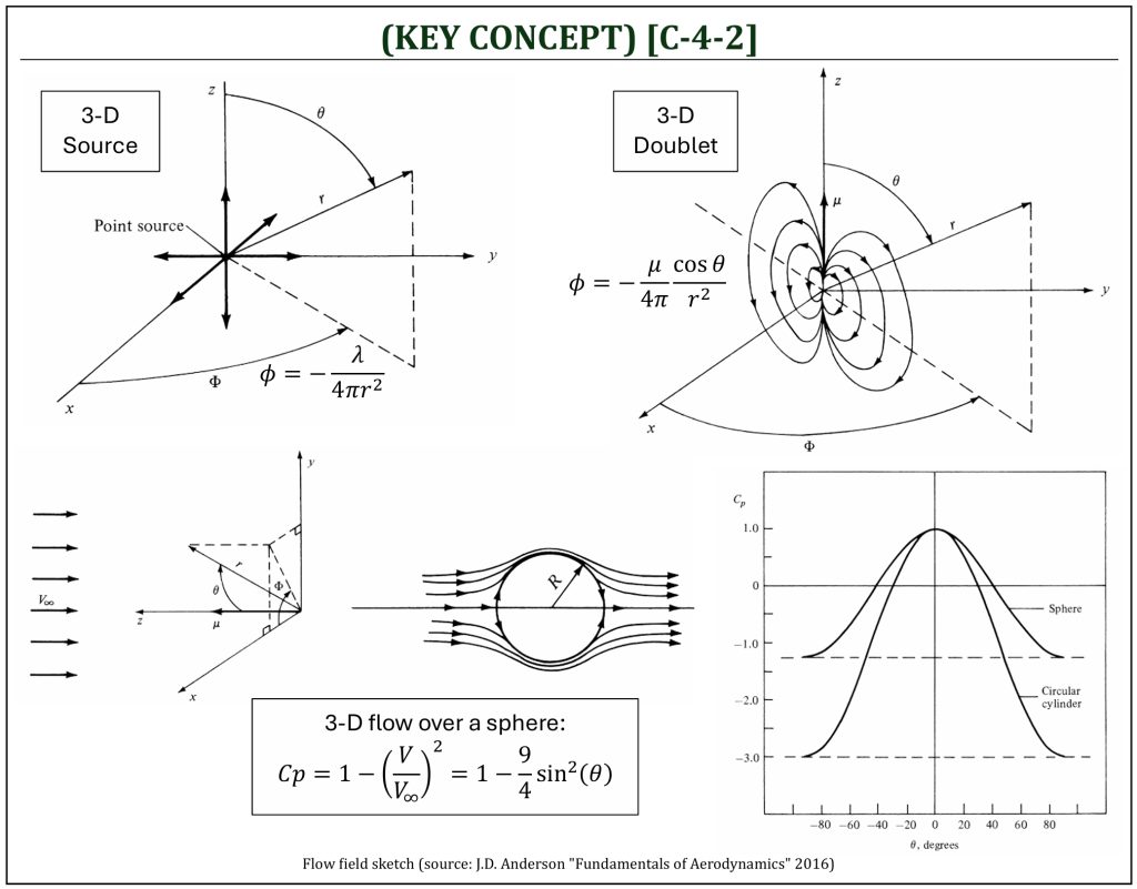
For a 3-D source (3-D elementary flow solution of Laplace’s equation), the velocity potential is given as:

$\phi = - \frac{C}{r}\ \ \ \ \ (\text{C is a constant})$

The velocity field is, therefore, given by:

$\overrightarrow{V} = \nabla\phi = \frac{C}{r^{2}}{\widehat{e}}_{r}$

The velocity components in spherical coordinate system ( $r,\theta,\Phi$ ) can be expressed, such that:

$V_{r} = \frac{C}{r^{2}},\ \ \ \ \ V_{\theta} = 0,\ \ \ \ \text{and}\ \ \ \ \ V_{\Phi} = 0$

Let us consider a sphere of radius $r$ . On the surface of the sphere, the velocity is a constant value, such that:

$V_{r} = \frac{C}{r^{2}}$

and is normal to the surface. From here, it is possible to define the constant ( $C$ ):

$\lambda = \frac{C}{r^{2}}4\pi r^{2} = 4\pi C\ \ \ \ \text{or}\ \ \ \ \ C = \frac{\lambda}{4\pi}$

where, $\lambda$ is called the “source strength.”

In conclusion, the flow field on the surface of the sphere of radius $r$ , induced by a 3-D source is:

$V_{r} = \frac{\lambda}{4\pi r^{2}}\ \ \ \ \text{and}\ \ \ \ \phi = - \frac{\lambda}{4\pi r}$

Now, let’s Consider a sink and source of equal but opposite strength located at points O and A. The distance between the source and sink is $l$ . Consider an arbitrary point $P$ located at distance $r$ from the sink and a distance $r_{1}$ from the source. The velocity potential at $P$ can be given from the equation of source as:

$\phi = - \frac{\lambda}{4\pi}\left( \frac{1}{r_{1}} - \frac{1}{r} \right) = - \frac{\lambda}{4\pi}\frac{r - r_{1}}{r\ r_{1}}$

Let the source approach the sink as their strength become infinite; that is: $l \rightarrow 0$ as $\lambda \rightarrow \infty$ . In the limit, as $l \rightarrow 0$ , $r - r_{1} \rightarrow l\cos(\theta)$ , and $r\ r_{1} \rightarrow r^{2}$ .

Thus, in the limit:

$\phi = - \lim_{\begin{matrix} l \rightarrow 0 \\ \lambda \rightarrow \infty \\ \end{matrix}}\left( \frac{\lambda}{4\pi}\frac{r - r_{1}}{r\ r_{1}} \right)^{\ } = - \frac{\lambda}{4\pi}\frac{l\cos(\theta)}{r^{2}}\ \ \ \ \text{or}\ \ \ \ \phi = - \frac{\mu}{4\pi}\frac{l\cos(\theta)}{r^{2}}$

Note that: $\mu = \lambda l$ is called the “doublet strength.” The velocity field in spherical coordinate system ( $r,\theta,\Phi$ ) can be expressed as:

$\overrightarrow{V} = \nabla\phi = V_{r}{\widehat{e}}_{r} + V_{\theta}{\widehat{e}}_{\theta} + V_{\Phi}{\widehat{e}}_{\Phi} = \frac{\mu}{2\pi}\frac{\cos(\theta)}{r^{3}}{\widehat{e}}_{r} + \frac{\mu}{4\pi}\frac{\sin(\theta)}{r^{3}}{\widehat{e}}_{\theta}\ \ \ \ \text{(NOTE)}\ V_{\Phi} = 0$

Now, superimposing 3-D doublet (strength $\mu$ and direction in the positive $z$ direction in 3-D cartesian coordinate system) and uniform flow (strength $V_{\infty}$ and direction in the negative $z$ direction) will construct a simulated flow over a sphere (similar to the 2-D flow over a circular cylinder, but now in 3-D flow field).

Uniform flow in negative $z$ direction induces the velocity field:

$\overrightarrow{V} = \nabla\phi = V_{r}{\widehat{e}}_{r} + V_{\theta}{\widehat{e}}_{\theta} + V_{\Phi}{\widehat{e}}_{\Phi} = - V_{\infty}\cos{(\theta){\widehat{e}}_{r}} + V_{\infty}\sin{(\theta){\widehat{e}}_{\theta}}\ \ \ \ \text{(NOTE)}\ V_{\Phi} = 0$

3-D doublet in positive $z$ direction induces the velocity field:

$\overrightarrow{V} = \nabla\phi = V_{r}{\widehat{e}}_{r} + V_{\theta}{\widehat{e}}_{\theta} + V_{\Phi}{\widehat{e}}_{\Phi} = \frac{\mu}{2\pi}\frac{\cos(\theta)}{r^{3}}{\widehat{e}}_{r} + \frac{\mu}{4\pi}\frac{\sin(\theta)}{r^{3}}{\widehat{e}}_{\theta}\ \ \ \ \text{(NOTE)}\ V_{\Phi} = 0$

By superimposing these, one can construct the flow field over a sphere:

$\overrightarrow{V} = \left\lbrack - V_{\infty}\cos(\theta) + \frac{\mu}{2\pi}\frac{\cos(\theta)}{r^{3}} \right\rbrack{\widehat{e}}_{r} + \left\lbrack V_{\infty}\sin{(\theta) +}\frac{\mu}{4\pi}\frac{\sin(\theta)}{r^{3}} \right\rbrack{\widehat{e}}_{\theta}\ \ \ \ \text{(NOTE)}\ V_{\Phi} = 0$

where,

$V_{r} = - V_{\infty}\cos(\theta) + \frac{\mu}{2\pi}\frac{\cos(\theta)}{r^{3}} = - \left( V_{\infty} - \frac{\mu}{2\pi r^{3}} \right)\cos(\theta)$

$V_{\theta} = V_{\infty}\sin(\theta) + \frac{\mu}{4\pi}\frac{\sin(\theta)}{r^{3}} = \left( V_{\infty} + \frac{\mu}{4\pi r^{3}} \right)\sin(\theta)\ \ \ \ \text{(NOTE)}\ V_{\Phi} = 0$

To find the stagnation point in the flow field, let $V_{r} = V_{\theta} = 0$ , then: $\theta = 0,\pi$ . Then from the requirement of $V_{r} = 0$ , it can be concluded that:

$V_{\infty} - \frac{\mu}{2\pi R^{3}} = 0\ \ \ \ \text{or}\ \ \ \ \ R = \left( \frac{\mu}{2\pi V_{\infty}} \right)^{\frac{1}{3}}$

$\text{Note that:}\ r=R\ \text{is the surface of the sphere}$

This will result in two stagnations points on the surface ( $r = R$ ) of the sphere:

$(r,\ \theta) = \left\lbrack \left( \frac{\mu}{2\pi V_{\infty}} \right)^{\frac{1}{3}},\ 0 \right\rbrack\ \ \ \ \text{and}\ \ \ \ \left\lbrack \left( \frac{\mu}{2\pi V_{\infty}} \right)^{\frac{1}{3}},\ \pi \right\rbrack$

Substituting $r = R$ into the expression for $V_{r}$ yields:

$V_{r} = - \left( V_{\infty} - \frac{\mu}{2\pi R^{3}} \right)\cos(\theta) - \left\lbrack V_{\infty} - \frac{\mu}{2\pi}\left( \frac{2\pi V_{\infty}}{\mu} \right) \right\rbrack\cos(\theta)$

$= - \left( V_{\infty} - V_{\infty} \right)\cos(\theta) = 0$

This means: $V_{r} = 0$ when $r = R$ for all values of $\theta$ and $\Phi$ . This is precisely the flow tangency condition ( $\overset{⃑}{V} \cdot \widehat{n} = 0$ ) for flow over a sphere of radius $R$ .

On the surface of the sphere ( $r = R$ ), the tangential velocity ( $V_{\theta}$ ) can be obtained as:

$V_{\theta} = \left( V_{\infty} + \frac{\mu}{4\pi R^{3}} \right)\sin(\theta)$

Note that $\mu = 2\pi R^{3}V_{\infty}$ , therefore:

$V_{\theta} = \left( V_{\infty} + \frac{1}{4\pi}\frac{2\pi R^{3}V_{\infty}}{R^{3}} \right)\sin(\theta) = \frac{3}{2}V_{\infty}\sin(\theta)$

Then, the pressure distribution on the surface of the sphere is:

$Cp = 1 - \left( \frac{V}{V_{\infty}} \right)^{2} = 1 - \left\lbrack \frac{3}{2}\sin(\theta) \right\rbrack^{2} = 1 - \frac{9}{4}\sin^{2}(\theta)$

If the pressure distribution over the surface of a sphere (3-D) is compared against cylinder (2-D), the pressure difference will be significantly less between the frontal and rearward surfaces. This is called the 3-D “relieving” effect. 3-D flow can move sideways (in addition to up-and-over, as well as down-and-under flows), and the pressure in the flow does not have to change so much. The flow in 3-D is “less stressed” due to the sideways flow (means that the pressure change is somewhat “relieved”).

Now, the concept of 2-D panel methods can easily be extended to the flow over 3-D bodies. General idea is that: covering the 3-D body with panels over which there is an unknown distribution of singularities (such as point sources, doublets, or vortices). With superposition against such a 3-D body with uniform flow (freestream, $V_{\infty}$ ), one can simulate a flow field around a 3-D body (conceptually, similar to the flow over a sphere).

References

Aerodynamics for Students by Auld & Srinivas (www.aerodynamics4students.com)
Fundamentals of Aerodynamics by J.D. Anderson, 5th ED, McGraw Hill, 2016
Aerodynamics for Engineers by J. J. Bertin & M. L. Smith, 3rd ED, Cambridge University Press, 1997
Aerodynamics for Engineering Students by E. L. Houghton & P. W. Carpenter, 4th ED, Edward Arnold, London, 1993

Software

The software applications are available (from www.aerodynamics4students.com) to build NACA airfoils in the form of standard ASCII text data files (a list of 2-D airfoil section coordinates). The format of these airfoil input data files is the de-facto standard for both thin airfoil theory and panel method programs. There is an initial header line, followed by a line giving the number of data points used to describe the airfoil and then pairs of surface coordinate points (x, y). The order of surface points is anti-clockwise, starting at the T.E. (trailing edge), going backward on the upper surface around the L.E. (leading edge) and then going forward along the lower surface to the T.E. From the surface coordinate data file, the program calculates a set of mean camber line coordinate points to be used for the mathematical analysis of airfoil sections:

NACA 2-D Airfoil Section Data Generator

The NACA airfoil section data can directly be applicable to simulate the aerodynamic characteristics of the given airfoil shape. Further, if any unique 2-D airfoil section is given as the section shape data, it can be simulated in a similar manner. The 2-D vortex panel method analysis can be done (mathematical analysis without viscous effects), but the limitations include: (i) compressibility effects are usually not included (may possibly be included by Prandtl-Glauert correction up to sonic speed, depending on the software application), (ii) usually no boundary layer effects (may possibly be included by a boundary layer solver with pressure gradient represented as a curved surfaces, and (iii) flow transition (laminar to turbulent) prediction may not be accurate. However, the vortex panel method based flow simulation software can be an extremely useful tool for a preliminary design of an aircraft at subsonic to transonic flight regime.

2-D Vortex Panel Method (including added boundary layer solver): SNR (Simulated-Not-Real) Virtual Wind Tunnel Laboratory

Media Attributions

If a citation and/or attribution to a media (images and/or videos) is not given, then it is originally created for this book by the author, and the media can be assumed to be under CC BY-NC 4.0 (Creative Commons Attribution-NonCommercial 4.0 International) license. Public domain materials have been included in these attributions whenever possible. Every reasonable effort has been made to ensure that the attributions are comprehensive, accurate, and up-to-date. The Copyright Disclaimer under Section 107 of the Copyright Act of 1976 states that allowance is made for purposes such as teaching, scholarship, and research. Fair use is a use permitted by copyright statute. For any request for corrections and/or updates, please contact the author.

License

Icon for the Creative Commons Attribution-NonCommercial 4.0 International License

2-D Source Panel Method

2-D Vortex Panel Method

3-D Potential Flow Analysis

References

Software

Media Attributions

License

Share This Book