B-1: Mathematics for Aerodynamics
Fundamentals of Mathematics for Aerodynamics
Shigeo Hayashibara
3-D Coordinate Systems
Cartesian and Cylindrical 3-D Coordinate Systems
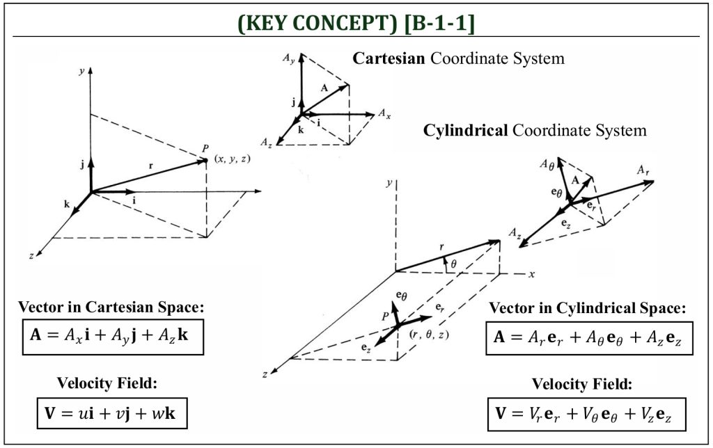
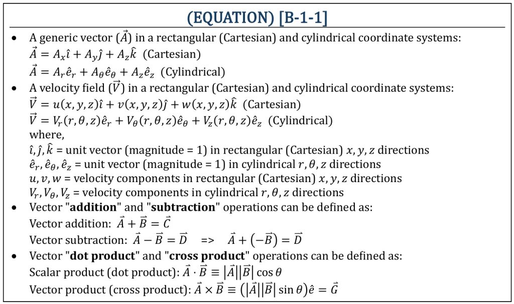
A flow field analysis of aerodynamics is often performed as vector field analysis. The velocity is a vector quantity in a flow field and represented as a “velocity field” in a 3-D coordinate system. There will be two commonly employed 3-D coordinates: (i) “rectangular” (Cartesian) and (ii) “cylindrical” coordinates. A vector quantity in a rectangular (Cartesian) and cylindrical coordinate systems can be described as follows:
Cartesian and Cylindrical 3-D Coordinate Systems
2-D Coordinate Systems
Cartesian and Polar 2-D Coordinate Systems
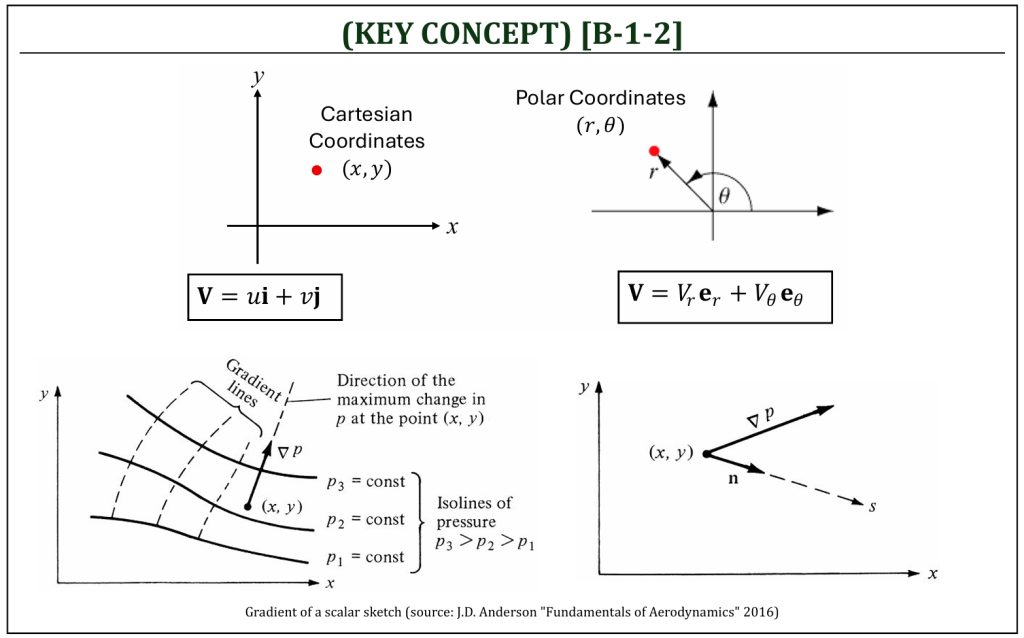
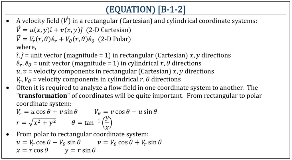
A 2-D flow field can also be defined in both (i) “rectangular” (Cartesian) and (ii) “polar” coordinates. A velocity field in a rectangular (Cartesian) and polar coordinate system can be described as follows:
Cartesian and Polar 2-D Coordinate Systems
A Gradient of a scalar
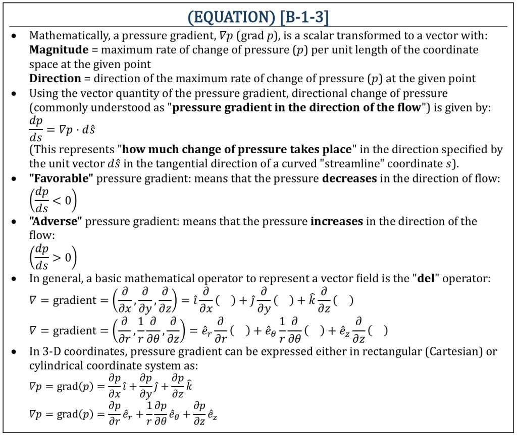
For a 2-D Cartesian coordinate system, a scalar property (pressure) is a function of spatial coordinates (x and y). In aerodynamics, often it is important to understand “how the pressure changes” in a certain direction; this is commonly called, the “pressure gradient.” A pressure gradient can be “favorable” (decreasing pressure in the direction) or “adverse” (increasing pressure in the direction). Generally speaking, an adverse pressure gradient causes flow “transition” (laminar to turbulent) as well as flow “separation.” Understanding the behavior of pressure gradient (i.e., the behavior of surface pressure change in a certain direction) is very important in aerodynamics. The shape of an airfoil is carefully designed to control the pressure gradient. A basic mathematical operator to represent a vector field is the “del” operator. Mathematically, the “del”  is an operator in vector calculous (also called the “nabla“). Taking the “del” operation (often also called “gradient” or “grad“) will turn a scalar property into a vector property.
A Gradient of a Scalar
Divergence and Curl of a vector field
Divergence and Curl
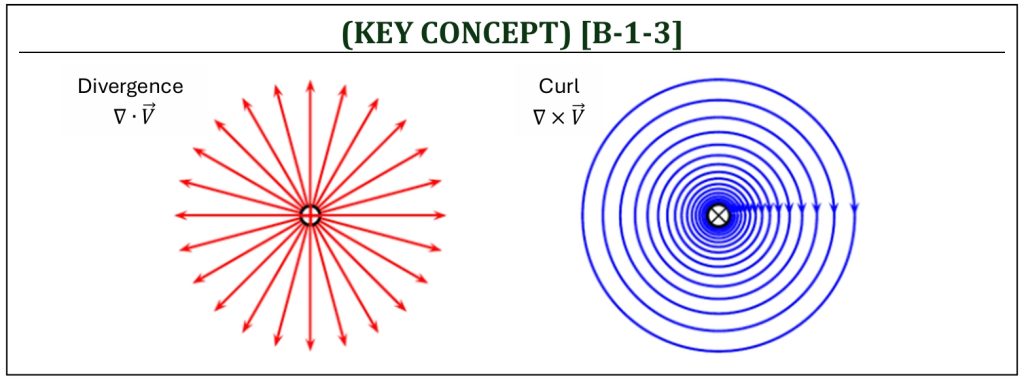
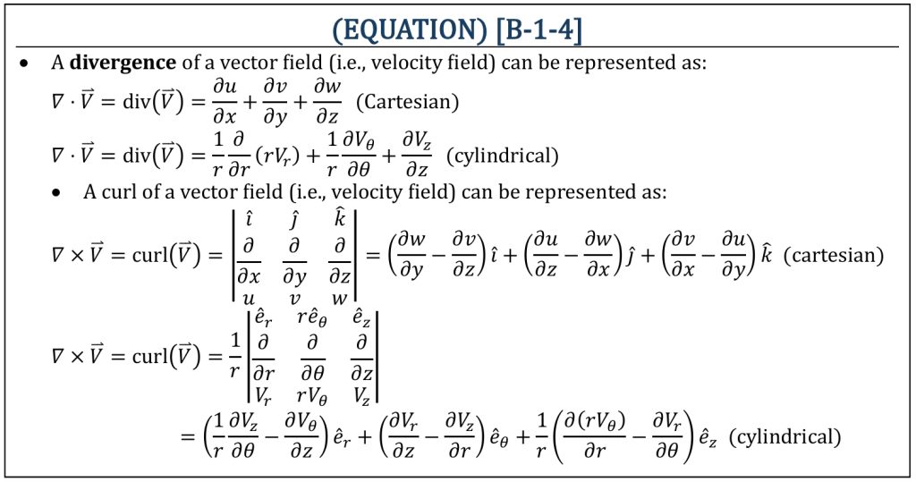
There are two fundamental mathematical vector field representations: (i) “divergence” and (ii) “curl” of a vector field. These actually mathematically represent vector field physics (including the physics of a flow field). Let us consider a “magnetic field” as an example. The “divergence” represents a magnetic field emanating from/into a source (either “+” or “–”). In fluid mechanics or aerodynamics (velocity field), a flow cannot suddenly appear or disappear at a single point; therefore, continuity principle is defined as “divergence of the velocity field is zero” that you can discover later in the potential (“ideal”) flow analysis. The flow field (velocity vector field) divergence is defined as a vector dot product (a scalar product) between the “del” operator and the “velocity” (vector property) of a flow field. It is often denoted by “div,” and mathematically represented in either rectangular (Cartesian) and cylindrical coordinates. The “curl” represents, for example, a velocity field in a circular pattern. In fluid mechanics or aerodynamics, this kind of flow field is commonly called a “vortex” type of flow. The flow field (velocity vector field) curl is defined as a vector cross product (a vector product) between the “del” operator and the “velocity” (vector property) of a flow field. It is often denoted by “curl,” and mathematically represented in either rectangular (Cartesian) and cylindrical coordinates.
Divergence and Curl of a Velocity Field
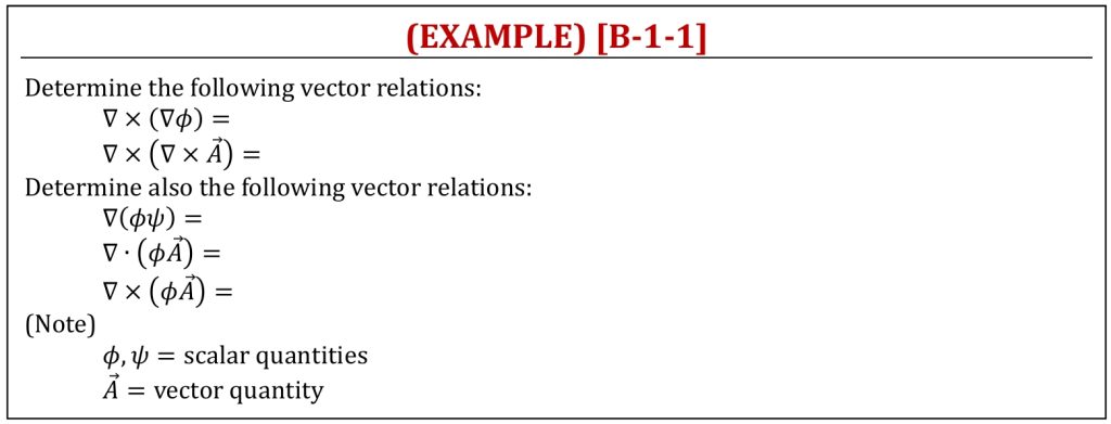
Non-Trivial Algebraic Rules of Vector Calculus
Line, Surface, and Volume Integrals
Line, Surface, and Volume Integrals
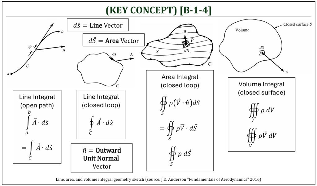
Mathematical integration of a differential expression of a flow field property is often important to analyze the flow field. Integration could be along a given line (1-D), over a given surface (2-D), and/or for a given volume (3-D). Recalling from A-3 (streamline coordinate system), it is often defined to specify directions “tangent” and “normal” with directional unit vectors (s and n). A vector quantity (i.e., velocity) dot products against these directional unit vectors can conveniently define directional components of the velocity at a given location.
In a similar manner, it is often convenient to define a “line vector” that is a vector in the tangential (parallel) direction of the given line at a given location (with magnitude ds). Also, it is often convenient to define an “area vector” that is a vector in the normal (perpendicular) direction of the given area at a given location (with magnitude dS). If a vector quantity (i.e., velocity) is involved, taking the dot product will set the positive (i.e., direction of the given line or outflow across the surface) or negative (i.e., opposite direction of the given line or inflow across the surface) sign convention of a flow field property.
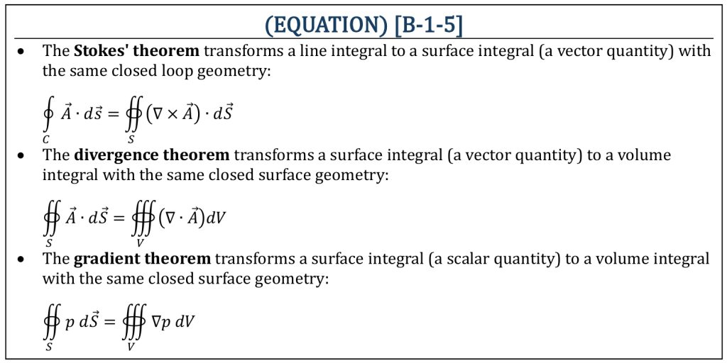
As it was already introduced in A-3 (derivation of Bernoulli’s equation), line, area, and volume integrals can be transformed (from 1-D to 2-D to 3-D integrals of a given flow field). These are called, Stokes’ theorem, divergence theorem, and gradient theorem of vector calculus.
Integral Transformation Operations
Conservation laws: (1) Conservation of mass (continuity)
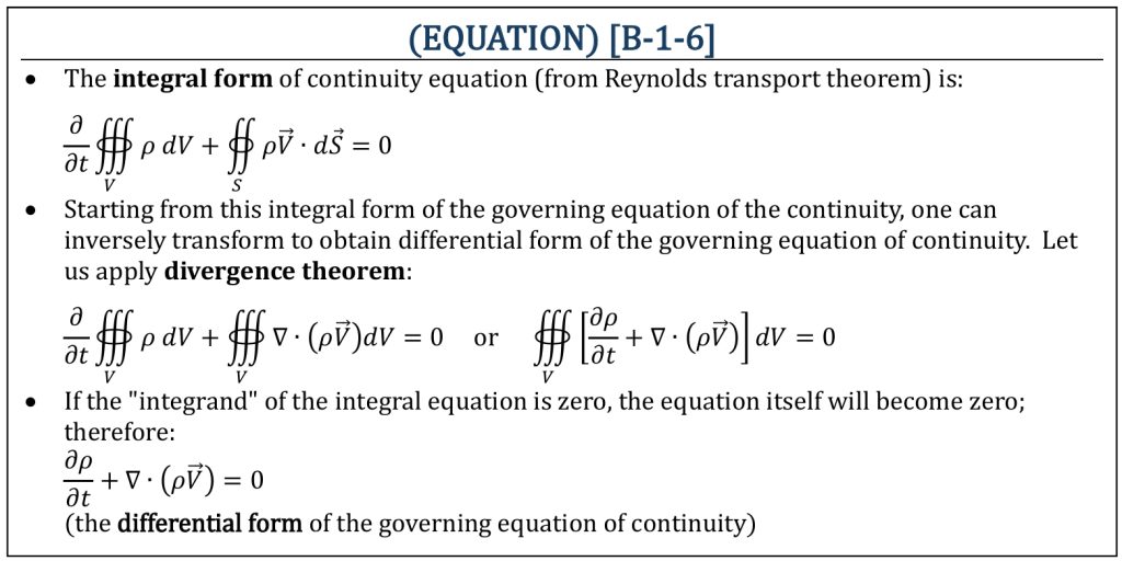
Recall, from A-3 (governing equation of continuity), Reynolds transport theorem (with a control volume) defines the integral form of continuity (governing equation for an Eulerian analysis). Applying the transformation (divergence theorem) can define the differential form of continuity (governing equation for a Lagragian analysis).
Conservation of Mass (Continuity)
Conservation laws: (2) Conservation of Linear Momentum
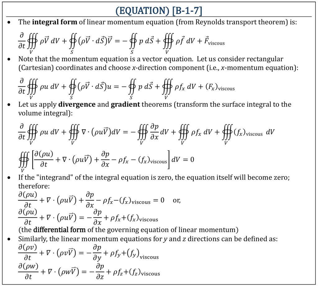
Recall (once again), from A-3 (governing equation of linear momentum), Reynolds transport theorem (with a control volume) defines the integral form of linear momentum (governing equation for an Eulerian analysis). Applying the transformation (divergence and gradient theorems) can define the differential form of linear momentum (governing equation for a Lagragian analysis).
Conservation of Linear Momentum
Substantial (material) derivative
Substantial (Material) Derivative of a Flow Field
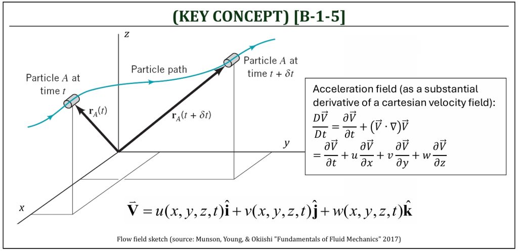
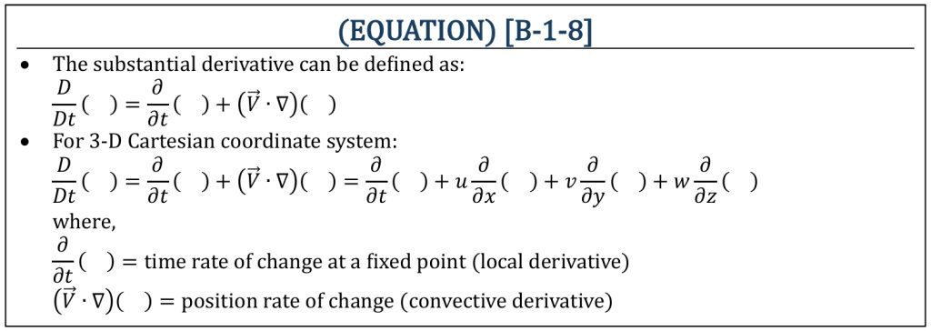
A flow field in aerodynamics usually means that there is “convection.” This means that the flow field properties (both scalar and vector) are transported throughout the flow field due to the presence of convection (i.e., existence of the velocity field). In order to understand the whole picture of flow field, therefore, one needs to keep track of two distinctively different “rates of changes” within the flow field . . . (i) how the property changes with respect of time at each location (“time rate of change” at each local location) and (ii) how the property changes with respect to location at each instant of time (“position rate of change” due to the presence of “convection“). Note that, for a steady flow field, the time rate of change becomes zero. The “total rate of change” (both “time” and “position”) of a fluid property (for example, an acceleration field) can be expressed mathematically in substantial (or often called, “total” or “material”) derivative.
Substantial (Total or Material) Derivative
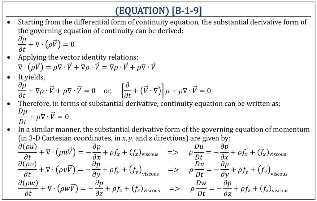
Now, governing equations (continuity and linear momentum) can be expressed in substantial derivative form to fully describe both “time” and “position” rate of changes within the given flow field.
Governing Equations in Substantial Derivative Form
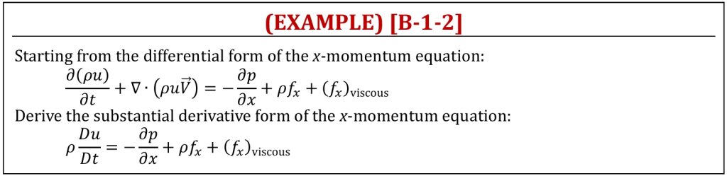
Substantial Derivative Form of Linear Momentum Equation
References
- Fundamentals of Aerodynamics by J.D. Anderson, 5th ED, McGraw Hill, 2016
- Aerodynamics for Engineers by J. J. Bertin & M. L. Smith, 3rd ED, Cambridge University Press, 1997
- Fundamentals of Fluid Mechanics by B. R. Munson, D. F. Yound, & T. H. Okiishi, 2nd ED, Wiley, 1994
- Aerodynamics for Engineering Students by E. L. Houghton & P. W. Carpenter, 4th ED, Edward Arnold, London, 1993
Media Attributions
If a citation and/or attribution to a media (images and/or videos) is not given, then it is originally created for this book by the author, and the media can be assumed to be under CC BY-NC 4.0 (Creative Commons Attribution-NonCommercial 4.0 International) license. Public domain materials have been included in these attributions whenever possible. Every reasonable effort has been made to ensure that the attributions are comprehensive, accurate, and up-to-date. The Copyright Disclaimer under Section 107 of the Copyright Act of 1976 states that allowance is made for purposes such as teaching, scholarship, and research. Fair use is a use permitted by copyright statute. For any request for corrections and/or updates, please contact the author.
