B-5: Conformal Mapping

Shigeo Hayashibara

B-5: Conformal Mapping

Joukowski Transformation (Conformal Mapping) Airfoil and Flow Field Simulation

Shigeo Hayashibara

From circular cylinder to an airfoil

Joukowski Airfoils and Flow Mapping

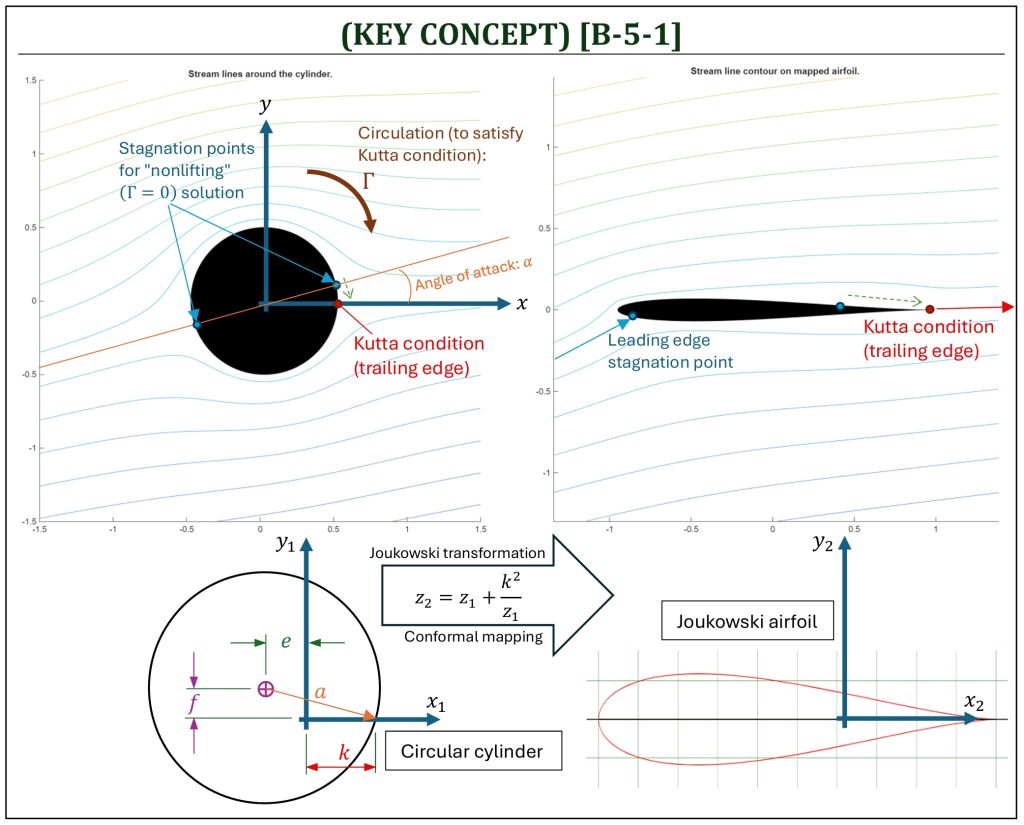
One of the ways of finding the flow patterns (streamlines), velocities, and pressures around a shape (similar to an “airfoil“) in a potential flow field is to apply a mathematical “conformal mapping” (called, “Joukowski transformation“) to the potential flow solution for a circular cylinder. The cylinder can be mathematically transformed (“mapped” from the original coordinate system to a transformed coordinate system) to simulate a variety of shapes including “airfoil-look-a-like” shapes, called a series of “Joukowski” airfoils. By knowing the derivative of the transformation used to perform the geometry mapping, along with the original solutions (i.e., stream function) around the circular cylinder, the potential flow field solution can be represented in the mapped flow field around a Joukowski airfoil.

A simple 2-D conformal mapping method, which produces a family of streamlined shapes (airfoil-look-a-like) is called the Joukowski transformation. The original circular cylinder (called, “z₁ flow field“) is mapped to a streamlined shape (called, “z₂ flow field“) by mathematical conformal mapping. The mapping is performed in a complex arithmetic transformation with z₁ (original) and z₂ (mapped) representing the coordinate space of each flow field coordinate, such that:

$z_{1} = x_{1} + i\y_{1}\ \ \ \ \text{and}\ \ \ \ \ z_{2} = x_{2} + i\y_{2}$

then, transformed by a conformal mapping, such that:

$z_{2} = z_{1} + \frac{k^{2}}{z_{1}}$

The transformation constant $k$ is used to control the stretching of the flow field. A small $k$ value will produce a near cylindrical shape with large thickness to chord ratio. A large $k$ value approaching the radius of the cylinder ( $a$ ) will produce a very thin streamlined shape. A value of $k = a$ will produce a flat plate. Values of $k$ greater than the radius of the cylinder produce mappings that are NOT conformal and hence do not represent valid flows.

By adjusting the center of the cylinder relative to the origin of flow field ( $z_{1}$ ), the mapped object can be made streamlined and curved (thus producing a “cambered” Joukowski airfoil section). To guarantee a valid airfoil shape the transformation constant must be adjusted to match the circular cylinder geometry, such that:

$(k + e)^{2} = a^{2} - f^{2}$

As the far-field (freestream) is undisturbed by the mapping, the freestream velocity ( $V_{\infty}$ ) for each coordinate space can be determined by the derivative of the transformation function, such that:

$\left| V_{2} \right| = \frac{\left| V_{1} \right|}{\left( \frac{dz_{2}}{dz_{1}} \right)}$

Note that the derivative of the transformation function is defined as:

$\frac{dz_{2}}{dz_{1}} = {1 - \frac{k^{2}}{z_{1}^{2}}}$

and then substituting for the transform function leads to:

$\left| V_{2} \right| = \frac{\left| V_{1} \right|}{1 - \frac{k^{2}}{z_{1}^{2}}}$

where $\left| V_{1} \right|$ is the magnitude of the velocity at a point in flow field ( $z_{1}$ ) and $\left| V_{2} \right|$ (or $V$ ) is the magnitude of the velocity at the mapped point in the airfoil flow field ( $z_{2}$ ).

The pressure coefficient on the surface of the streamlined shape in flow field ( $z_{2}$ ) can then be found by applying Bernoulli’s equation for inviscid incompressible flow, such that:

${C_{p}}_{2} = 1 - \frac{V_{2}^{2}}{V_{\infty}^{2}}$

For streamline shapes with sharp trailing edges, such as Joukowski airfoil sections, circulation must be added to the flow to obtain the correct lifting solution. The value of circulation applied to the cylinder in flow field ( $z_{1}$ ) should be specified so that a stagnation point is produced at the point of intersection of the rear of the cylinder and the x-axis. This trailing edge ( $z_{1}$ ) point maps to the trailing edge of the airfoil and when the correct amount of circulation is applied, the Kutta condition (i.e., vorticity = 0 at trailing edge) will be satisfied at the trailing edge of the airfoil in flow field ( $z_{2}$ ). This means the required amount of circulation is:

$\Gamma = 4\pi aV_{\infty}\sin(\alpha)$

where $a$ is the radius of the original circle and $\alpha$ is the stream angle of attack. Having obtained the correct flow pattern, the lift (per unit depth) can be calculated as a function of the amount of circulation applied, such that:

$Lift = \rho_{\infty}V_{\infty}\Gamma$

or, in terms of lift coefficient:

$c_{l} = \frac{\Gamma}{RV_{\infty}}$

Flat Plate Joukowski Transformation

Flat Plate (Thin Airfoil) Joukowski Transformation

KEY CONCEPT [B-5-2]

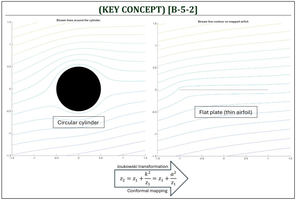
A Joukowski mapping can be used of known flow around a circular cylinder to predict flow over a flat plate airfoil at an angle of attack ( $\alpha$ ), where $k = a$ the radius of circle. The equation for the surface of the circle can be set in polar coordinates ( $z_{1} = ae^{i\theta}$ ), hence the equation for the surface of the plate can be found from the transformation:

$z_{2} = ae^{i\theta} + \frac{a^{2}}{ae^{i\theta}} = {ae}^{i\theta} + {ae}^{- i\theta} = a\left( e^{i\theta} + e^{- i\theta} \right)$

Note that the complex function $e^{i\theta}$ can alternatively be expressed as:

$e^{i\theta} = \cos{(\theta) + i\sin(\theta)}\ \ \ \ \text{and}\ \ \ \ \ e^{- i\theta} = \cos{(\theta) - i\sin(\theta)}$

then:

$z_{2} = a\left\lbrack \cos{(\theta) + i\sin{(\theta) + \cos{(\theta) - i\sin(\theta)}}} \right\rbrack = 2a\cos(\theta)$

Therefore, from the definition ( $z_{2} = x_{2} + iy_{2}$ ), it is concluded that:

$x_{2} = 2a\cos(\theta)\ \ \ \ \text{and}\ \ \ \ \ y_{2} = 0$

Now, it is important to apply a correct Kutta condition (the condition that the trailing edge of the flat plate must be the stagnation point), the required circulation is given as:

$\Gamma = 4\pi aV_{\infty}\sin(\alpha)$

This means rotation (i.e., flow field circulation) is added to the circle sufficient to move the rear stagnation point to the location that maps to the trailing edge of the plate. The velocity ( $V_{1}$ ) at any point on the surface of the circle( $z_{1}$ ) will be the sum of the standard circle flow, rotated by an angle ( $\alpha$ ) and the contribution from the vortex on the origin, such that:

$V_{1} = 2V_{\infty}\sin{(\theta - \alpha) + \frac{\Gamma}{2\pi a}} = 2V_{\infty}\sin{(\theta - \alpha) + \frac{4\pi aV_{\infty}\sin(\alpha)}{2\pi a}$

$= 2V_{\infty}\sin{(\theta - \alpha) + 2V_{\infty}\sin(\alpha)}}$

note that:

$\sin{(\theta - \alpha) = \sin{(\theta)\cos{(\alpha) - \cos{(\theta)\sin(\alpha)}}}}$

therefore:

$V_{1} = 2V_{\infty}\left\lbrack \sin{(\theta)\cos(\alpha)} - \cos{(\theta)\sin{(\alpha) + \sin(\alpha)}} \right\rbrack$

The velocity on the surface of the plate will be based on circle flow velocity and the absolute value of the derivative of the transformation function:

$V_{2} = \frac{V_{1}}{\left| \frac{dz_{2}}{dz_{1}} \right|}$

The derivative can be evaluated as:

$\frac{dz_{2}}{dz_{1}} = 1 - \frac{k^{2}}{z_{1}^{2}} = 1 - \frac{a^{2}}{a^{2}e^{2i\theta}} = 1 - e^{- 2i\theta} = 1 - \left\lbrack \cos{(2\theta) - i\sin(2\theta)} \right\rbrack$

hence,

$\frac{dz_{2}}{dz_{1}} = \cos^{2}(\theta) + \sin^{2}(\theta) - \cos^{2}(\theta) + \sin^{2}(\theta) + 2i\cos(\theta)\sin(\theta)$

$= 2\sin{(\theta)\left\lbrack \sin{(\theta) + i\cos(\theta)} \right\rbrack}$

The magnitude is:

$\left| \frac{dz_{2}}{dz_{1}} \right| = 2\sin(\theta)$

The velocity on the flat plate can then be calculated as:

$V_{2} = \frac{2V_{\infty}\left\lbrack \sin{(\theta)\cos(\alpha)} - \cos{(\theta)\sin{(\alpha) + \sin(\alpha)}} \right\rbrack}{2\sin(\theta)}$

$= V_{\infty}\left\{ \cos{(\alpha) + \sin{(\alpha)\left\lbrack 1 - \cot(\theta) \right\rbrack}} \right\}$

or,

$V_{2} = V_{\infty}\left\lbrack \cos{(\alpha) + \sin{(\alpha)\tan\left( \frac{\theta}{2} \right)}} \right\rbrack$

If only small angles of attack are considered so that no flow separation occurs:

$\alpha$ is small, $\cos{(\alpha) \approx 1}$ , and $\sin{(\alpha) \approx \alpha}$ then,

$V_{2} = V_{\infty}\left\lbrack 1 + \alpha\tan\left( \frac{\theta}{2} \right) \right\rbrack$

Surface pressure coefficient will be found by applying the incompressible version of Bernoulli equation,

$Cp = 1 - \frac{V_{2}^{2}}{V_{\infty}^{2}} = 1 - \left\lbrack 1 + \alpha\tan\left( \frac{\theta}{2} \right) \right\rbrack^{2} = - 2\alpha\tan{\left( \frac{\theta}{2} \right) - \alpha^{2}\tan^{2}\left( \frac{\theta}{2} \right)}$

The pressure distribution over the airfoil can be observed by looking at upper surface ( $\theta$ ) and the lower surface ( $- \theta$ ) pressure coefficients. $Cp$ at the trailing edge ( $\theta = 0$ ) is zero. On the upper surface the coefficient becomes more and more negative towards the leading edge ( $\theta = \pi$ ), where it produces infinite suction (low pressure).

On the lower surface going forward, $\tan\left( - \frac{\theta}{2} \right)$ is positive and $\tan{\left( \frac{\theta}{2} \right) >}\tan^{2}\left( \frac{\theta}{2} \right)$ so initially the coefficient becomes more positive. This continues up to the point when $V_{2} = 0$ , the stagnation point near the leading edge of the flat plate, where $\alpha\tan{\left( - \frac{\theta}{2} \right) = - 1}$ and $Cp = 1$ .

In front of this, $\alpha\tan{\left( \frac{\theta}{2} \right) > 1}$ and $\alpha\tan{\left( \frac{\theta}{2} \right) < \alpha^{2}\tan^{2}\left( \frac{\theta}{2} \right)}$ so the coefficient reduces to zero and then becomes more and more negative, eventually equaling the infinite suction (low pressure) at the leading edge.

The resultant of upper and lower surface pressures pushing on the surface of the plate will result in a normal force. The component of this normal force perpendicular to the stream will be the lift. For small angles of attack: $\cos{(\alpha) \approx 1}$ , thus the normal force is the same as the lift. Lift can then be calculated as the sum of pressure forces acting normal to the surface.

$Lift = \int_{0}^{c}\left( P_{lower} - P_{upper} \right)dx$

where for 2-D sections, the force acts on a 1-unit depth of wing (unit span). The lift coefficient will then be,

$c_{l} = \frac{Lift}{\frac{1}{2}\rho V_{\infty}^{2}} = \int_{0}^{1}{\frac{P_{lower} - P_{upper}}{\frac{1}{2}\rho V_{\infty}^{2}}\left( \frac{dx}{c} \right) = \int_{0}^{1}\left( {Cp}_{lower} - {Cp}_{upper} \right)}\left( \frac{dx}{c} \right)$

Substituting for the previous expression for pressure coefficient,

$c_{l} = \int_{0}^{1}\left\lbrack - \alpha\tan\left( - \frac{\theta}{2} \right) - \alpha^{2}\tan^{2}{\left( - \frac{\theta}{2} \right) + \alpha\tan\left( \frac{\theta}{2} \right) + \alpha^{2}\tan^{2}\left( \frac{\theta}{2} \right)} \right\rbrack\left( \frac{dx}{c} \right)$

or,

$c_{l} = \int_{0}^{1}\left\lbrack \alpha\tan\left( \frac{\theta}{2} \right) - \alpha^{2}\tan^{2}{\left( \frac{\theta}{2} \right) + \alpha\tan\left( \frac{\theta}{2} \right) + \alpha^{2}\tan^{2}\left( \frac{\theta}{2} \right)} \right\rbrack\left( \frac{dx}{c} \right)$

$= \int_{0}^{1}\left\lbrack 2\alpha\tan\left( \frac{\theta}{2} \right) \right\rbrack\left( \frac{dx}{c} \right)$

From the mapping geometry,

$dx = dx_{2} = \frac{dx_{2}}{d\theta} = - 2a\sin{(\theta)d\theta}$

In addition,

$c \approx 4a$

$\theta = \pi\ \ when\ \ \frac{x}{c} = 0\ \ \ \ \text{and}\ \ \ \ \ \theta = 0\ \ when\ \ \frac{x}{c} = 1$

Therefore,

$c_{l} = \int_{\pi}^{0}{2\alpha\tan{\left( \frac{\theta}{2} \right)\frac{- 2a\sin(\theta)}{4a}}d\theta} = \int_{0}^{\pi}{2\alpha\tan{\left( \frac{\theta}{2} \right)\sin{(\theta)d\theta} = 2\pi\alpha}}$

As the lowest pressure region is toward the front, a pitching moment will be created about the center of the flat plate by the distribution of lift over the chord of the flat plate. There will be a balance point toward the leading edge of the flat plate, and this can be calculated by summing the moments caused by individual lift elements along the chord. The moment about the leading edge ( $x = 0$ ) is:

$m_{l.e.} = \int_{LE}^{TE}{- \left( P_{lower} - P_{upper} \right)xdx}$

${c_{m}}_{l.e.} = \frac{m_{l.e.}}{\frac{1}{2}\rho V_{\infty}^{2}Sc} = \int_{0}^{1}{- \left( {Cp}_{lower} - {Cp}_{upper} \right)\left( \frac{x}{c} \right)\left( \frac{dx}{c} \right)}$

by definition, the pitching moment is positive nose up. Hence the negative sign for leading edge moment coefficient. In this case the moment arm can also be found from the geometry of the transformation ( $x \approx x_{2} + 2a$ ), such that:

$x = 2a\cos{(\theta) + 2a}$

so, the substitution can be made for pressure coefficient, moment arm and integration variable.

${c_{m}}_{l.e.} = \int_{0}^{1}{\left\lbrack - \alpha\tan{\left( - \frac{\theta}{2} \right) - \alpha^{2}\tan^{2}{\left( - \frac{\theta}{2} \right) +}}\alpha\tan{\left( \frac{\theta}{2} \right)$

$+ \alpha^{2}\tan^{2}\left( \frac{\theta}{2} \right)} \right\rbrack\frac{2a + 2a\cos(\theta)}{c}\frac{dx}{c}}$

${c_{m}}_{l.e.} = \int_{\pi}^{0}{\left\{ 2\alpha\tan{\left( \frac{\theta}{2} \right)\left\lbrack 1 + \cos(\theta) \right\rbrack} \right\}\frac{2a}{4a}\frac{- 2a\sin(\theta)}{4a}d\theta}$

$= \int_{0}^{\pi}{\left\{ \frac{1}{2}\alpha\tan\left( \frac{\theta}{2} \right)\left\lbrack 1 + \cos(\theta) \right\rbrack \right\}\sin{(\theta)d\theta}}$

In conclusion:

${c_{m}}_{l.e.} = - \left( \frac{\pi}{2} \right)\alpha$

This can be used to predict pitching moment about the standard reference point at the quarter chord location.

${c_{m}}_{\frac{c}{4}} = {c_{m}}_{l.e.} + c_{l}\frac{0.25c}{c} = {c_{m}}_{l.e.} + \frac{c_{l}}{4} = - \frac{\pi}{2} + \frac{2\pi\alpha}{4} = 0$

Hence, the center of pressure is at the $\frac{1}{4}$ chord (quarter chord) location on the flat plate.

As the quarter chord moment coefficient ( ${c_{m}}_{\frac{c}{4}}$ ) is independent of angle of attack ( $\alpha$ ), the aerodynamic center will also be at the quarter chord.

Summary: Joukowski Transformation

Flat Plate

If the transformation constant is set to be equal to the radius of the circle ( $k = a$ ) and no center shift is used, the circle maps simply to a flat plate. By applying the velocity mapping and Bernoulli’s relationships, the pressure field on the plate can be predicted (and hence the lift, drag and moment can be calculated). Analysis of a Joukowski transformation to a flat plate airfoil leads to the following standard results:

$c_{l} = 2\pi\alpha$

$c_{m,c/4} = 0$

$c_{d} = 0$

General Joukowski Airfoil Solution

While Joukowski airfoils are relatively simple to create and analyze, they are relatively crude in terms of performance. The geometric properties of this family can be described by the following approximations:

$\text{Maximum thickness:}\ t_{\max} \approx \frac{3\sqrt{3}}{4}\left( \frac{e}{a} \right)$

$\text{Maximum camber height:}\ h_{\max} \approx \frac{f}{2k}$

The location of the maximum thickness is always at the 30% chord location and the location of the maximum camber point is always 50% chord. This arrangement promotes early boundary layer transition and hence moderately higher drag. The cusped trailing edge is extremely thin and impractical for real construction purposes.

The performance due to camber is modified such that,

$c_{l} = 2\pi\left( \alpha - \alpha_{0} \right) = 2\pi\alpha + {c_{l}}_{0}$

$c_{m,c/4} < 0$

References

Aerodynamics for Students by Auld & Srinivas (www.aerodynamics4students.com)
Fundamentals of Aerodynamics by J.D. Anderson, 5th ED, McGraw Hill, 2016
Aerodynamics for Engineers by J. J. Bertin & M. L. Smith, 3rd ED, Cambridge University Press, 1997
Aerodynamics for Engineering Students by E. L. Houghton & P. W. Carpenter, 4th ED, Edward Arnold, London, 1993

Software

The software application is available (from www.aerodynamics4students.com) to construct and display flow patterns (streamlines), pressures, and list coordinate data for these transformed airfoil sections:

Joukowski Airfoil Generator and Flow Field Analyzer

Media Attributions

If a citation and/or attribution to a media (images and/or videos) is not given, then it is originally created for this book by the author, and the media can be assumed to be under CC BY-NC 4.0 (Creative Commons Attribution-NonCommercial 4.0 International) license. Public domain materials have been included in these attributions whenever possible. Every reasonable effort has been made to ensure that the attributions are comprehensive, accurate, and up-to-date. The Copyright Disclaimer under Section 107 of the Copyright Act of 1976 states that allowance is made for purposes such as teaching, scholarship, and research. Fair use is a use permitted by copyright statute. For any request for corrections and/or updates, please contact the author.

License

Icon for the Creative Commons Attribution-NonCommercial 4.0 International License