Representation of streamlines

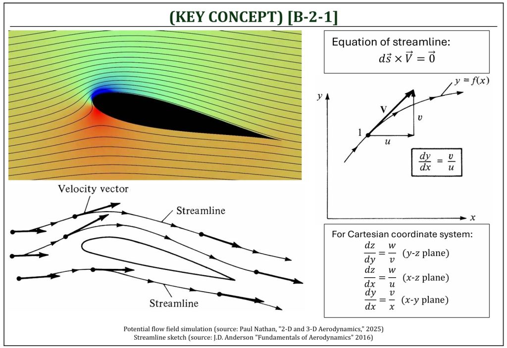
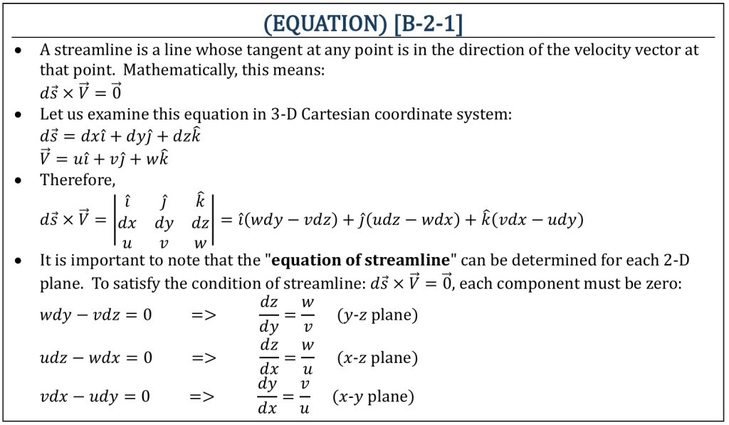
A streamline is a line whose tangent at any point is in the direction of the velocity vector at that point.  A streamline can be mathematically represented by setting the cross product between the line vector of a given streamline (pointing the tangential direction for that location) and the velocity at that location along the given streamline equal to zero.

representation of Viscous Effects

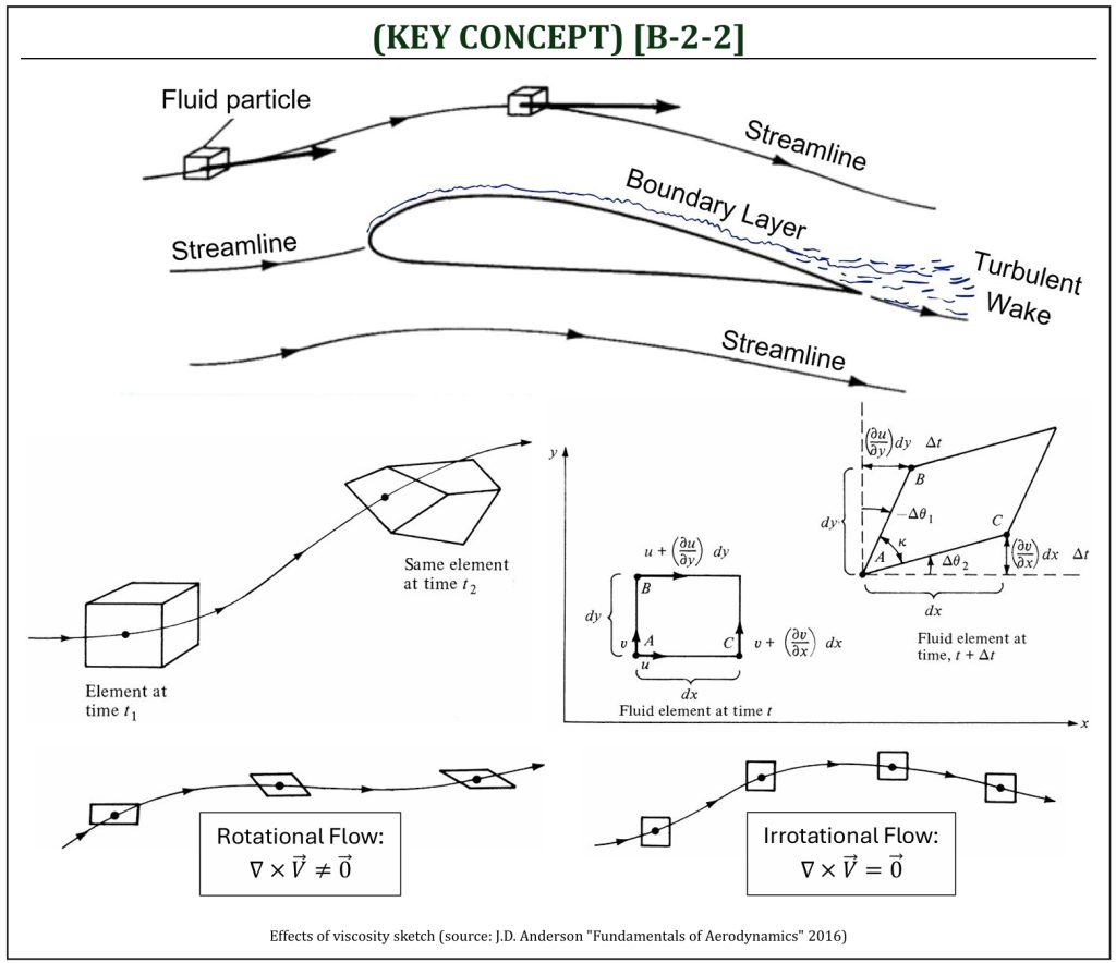
As a fluid element moves along a streamline, obviously it “translates” from one position to another (can be represented, simply, by the velocity of a flow field).  Also, the element “rotates” and “distorts” as it moves.  This combined rotation + distortion (i.e., angular deformation) can mathematically be represented by the “angular velocity” of a flow field.  The presence of “viscosity” causes both “rotation” and “angular deformation,” and the flow field is defined as “rotational flow.”  If the viscosity within the flow field is ignored (“inviscid” flow), the motion of a fluid element can be simplified only for “translation”: this is called, “irrotational flow.”

When a fluid element rotates (and also being distorted due to its rotation), the magnitude of rotation of an element (in Cartesian x-y plane) can be defined by the angular velocity.  Note that the angular velocity (rotation) can mathematically be related to the rate of shear strain (angular deformation); such that: (traveling distance, due to velocity difference) = (arc length, due to the rotation of the edge of an element).

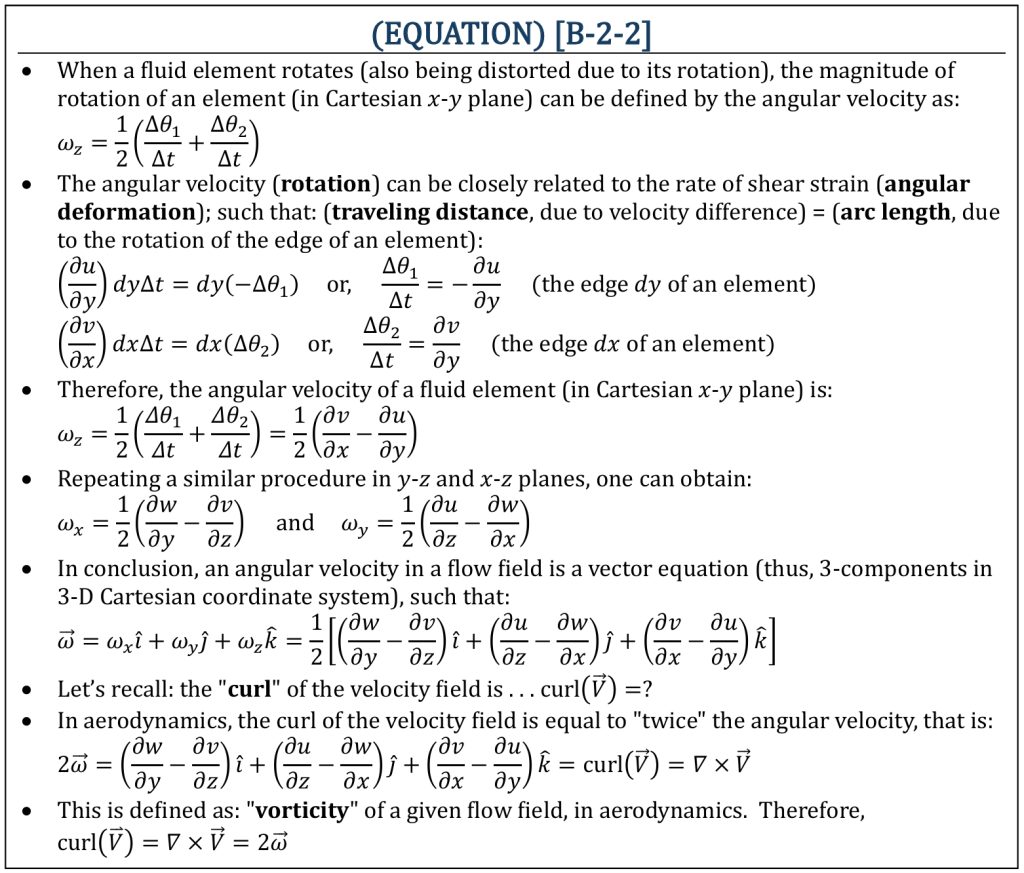
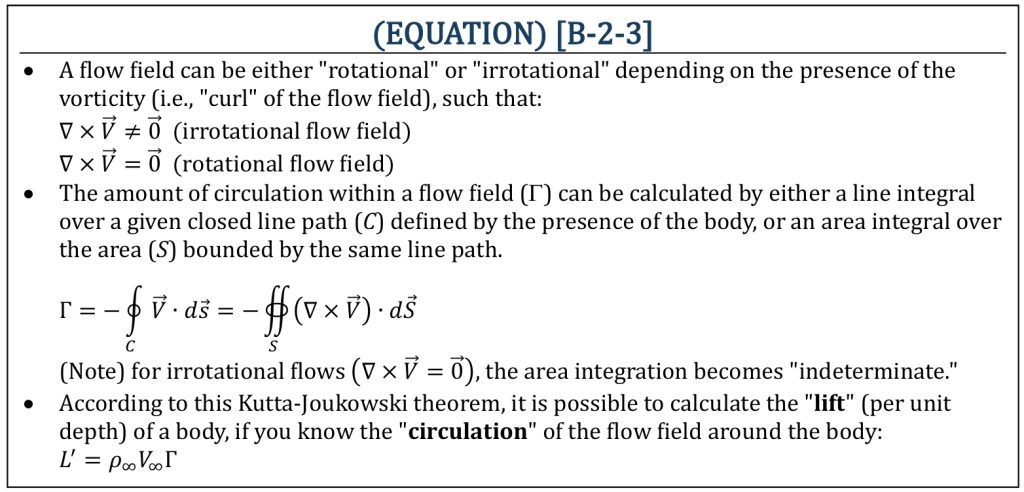
We can categorize two fundamentally different types of flow field of aerodynamics, in terms of the presence of vorticity in the flow field: if the flow field vorticity is not zero, the flow field is called “rotational.”  This implies that the fluid elements have a finite angular velocity.  If the flow field vorticity is zero at every point in a flow, the flow field is called “irrotational.”  This implies that the fluid elements have no angular velocity; rather, their motion through space is a pure translation.

If the flow field is irrotational, the governing equation of the flow field can be significantly simplified.  As a result, one can model and analyze basic behaviors of the flow field by algebraic mathematical formulations.  If the flow field is: (i) steady, (ii) no body force, (iii) inviscid, (iv) incompressible, and (v) irrotational (because “inviscid“), then the flow field is called, “ideal” (or “potential“) flow field.  The ideal (or potential) flow fields can be analyzed mathematically (100% pure theory).  This is commonly referred to: “theoretical aerodynamics” by “potential flow field analysis.”

Circulation theory of aerodynamics

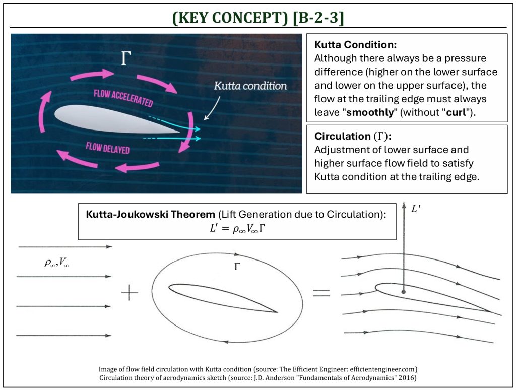
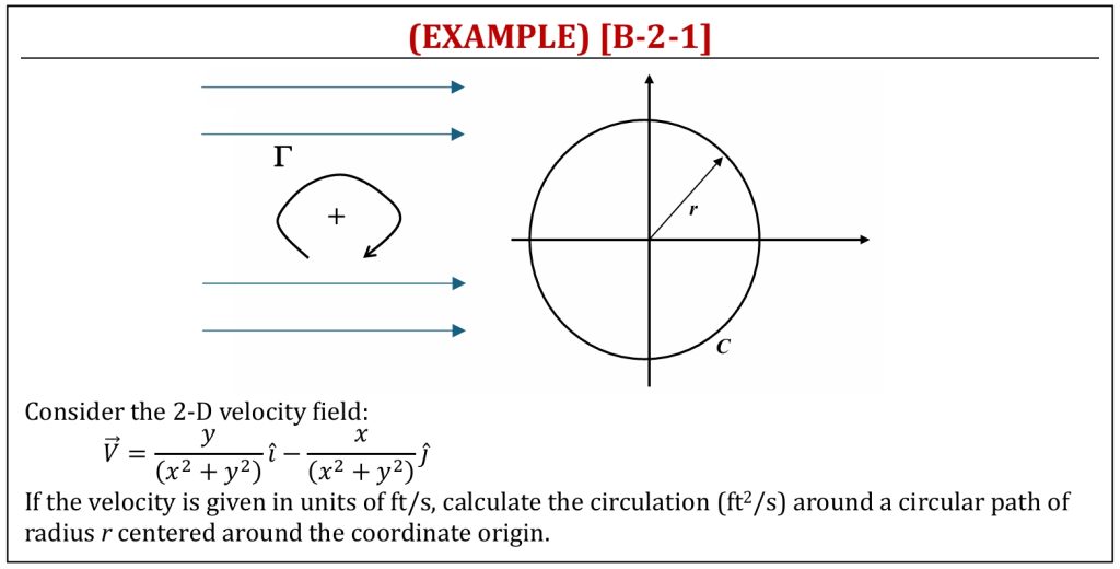
A flow field may have a “circulation.”  A circulation is a very fundamental tool, in theoretical aerodynamics, to determine an aerodynamic lift within an ideal (or potential) flow field.  The presence of a body (such as an “airfoil”) within a uniform flow will cause a “circulation” within the given flow field.  If we calculate the amount of circulation within the flow field, we can calculate the amount of “lift” developed on the body.  Mathematically, the amount of circulation within a flow field can be calculated by either a line integral over a given closed line path (C) defined by the presence of the body, or an area integral over the area (S) bounded by the same line path.

The “circulation theory” is a general classical mathematical formulation to predict the aerodynamic lift of a body within a given flow field.  This is a very well-established mathematical model-based flow field analysis of an ideal (or potential) flow field (pure theory).  In circulation theory, it is predicted that an aerodynamic lift is generated due to the time rate of change of airflow in the downward direction (change of the momentum), due to the amount of circulation in the flow field (caused by the presence of a body within the flow field).  The “Kutta-Joukowski” theorem is the most important outcome of the circulation theory.  If a circulation of a 2-D flow field is known, the lift per unit depth of a lifting body can be calculated from the freestream velocity and density of the flow field.  According to this Kutta-Joukowski theorem, it is possible to calculate the “lift” (per unit depth) of a body, if you know the “circulation” of the flow field around the body (which is generated due to the presence of the body itself in the flow field).

Ideal Flow field solutions (potential flow analysis)

As an ideal (potential) flow field is mathematically analyzed, we can employ 2 mathematical field functions: (i) “stream function” and (ii) “velocity potential.”

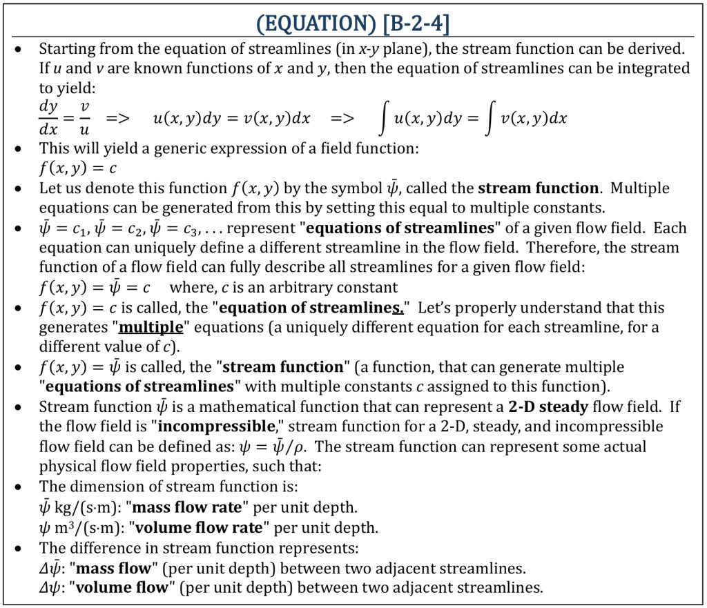
A “stream function” (ψ) is a 2-D mathematical field function of a potential flow field.  Starting from the equation of streamlines (in x-y plane), the stream function can be derived.  If u and v are known functions of x and y, then the equation of streamlines can be integrated to yield a mathematical field function (stream function).

A similar to the stream function, a “velocity potential” (ϕ) is also a mathematical field function to represent steady, incompressible, and irrotational flow field.  A flow field that can be described by a velocity potential is called, a “potential flow field.”

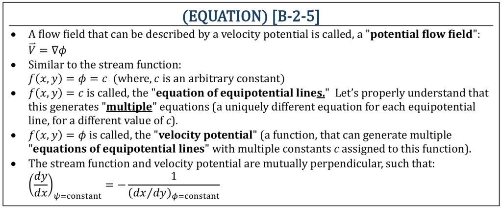
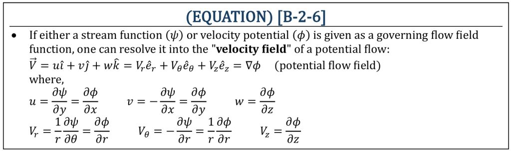
Drawing a series of lines, mathematically, within a given flow field (governed by either a stream function or a velocity potential) will represent either “streamlines” (lines of constant ψ‘s) or “equipotential lines” (lines of constant ϕ‘s).  These lines are mutually perpendicular to each other.  If either a stream function or velocity potential is given as a governing flow field function, one can resolve it into the “velocity field” of a potential flow.

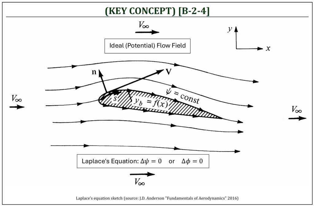
The flow field that can define “velocity potential” (steady, no body force, incompressible, inviscid, and irrotational flow field) is called the “potential” flow field.  This is also called the “ideal” flow field (as the flow field can be analyzed purely mathematically).  An ideal flow field is governed by a partial differential equation (PDE), called the “Laplace’s equation.”  Theoretical aerodynamics is essentially an analysis, attempting to solve Laplace’s equation for an ideal flow field.  For an “ideal” flow field, under multiple assumptions, equations are simplified.  For example, let us consider one of the governing equations of a flow field, “x-momentum” equation.

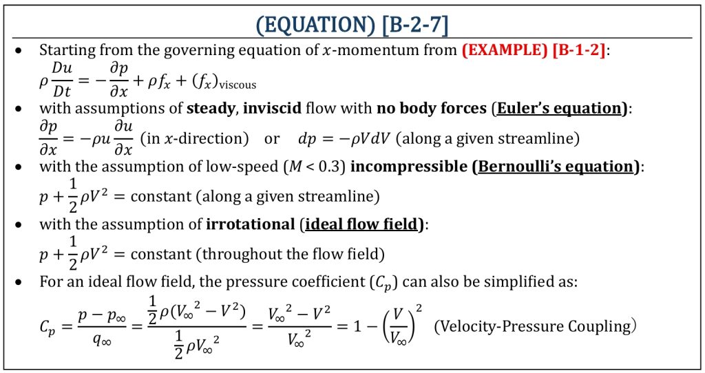
As clearly be seen for an ideal flow field, if the velocity field is given, one can easily calculate the distribution of pressure (on any surface) within the flow field.  This is called, the “velocity-pressure coupling.”  The Laplace’s equation is a second-order linear partial differential equation that governs the “ideal” (i.e., “potential“) flow field.  Let us hereby prove that, indeed, the Laplace’s equation is the equation that can be defined for a given flow field under certain conditions (assumptions).

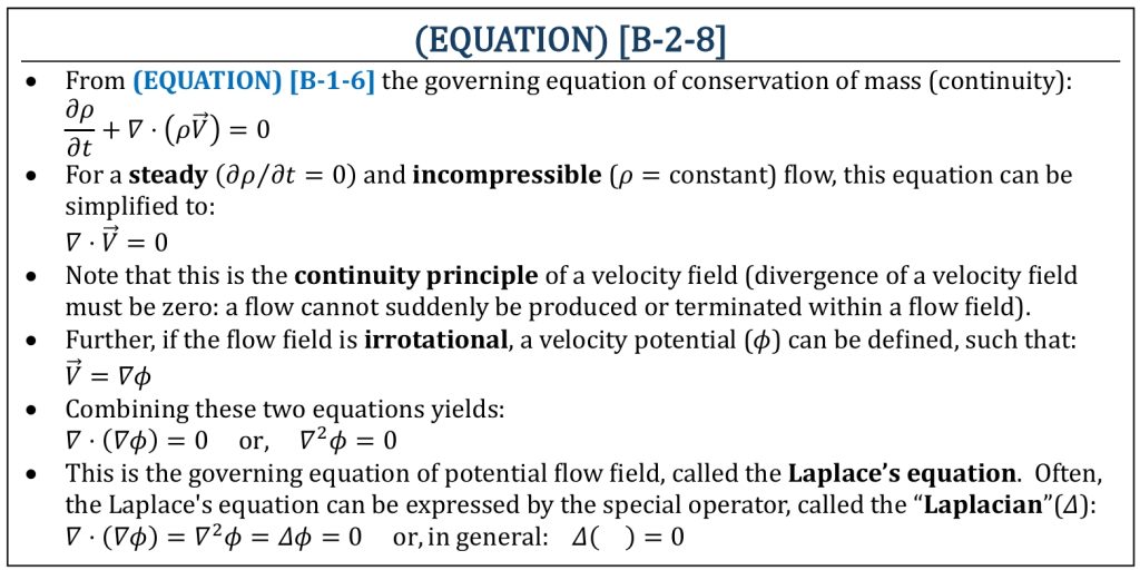
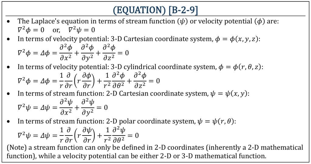
Laplace’s equation can be represented in both 2-D and 3-D rectangular (Cartesian) and cylindrical (or polar) coordinates in terms of either the stream function ψ or the velocity potential ϕ (as a governing function) of the given flow field.

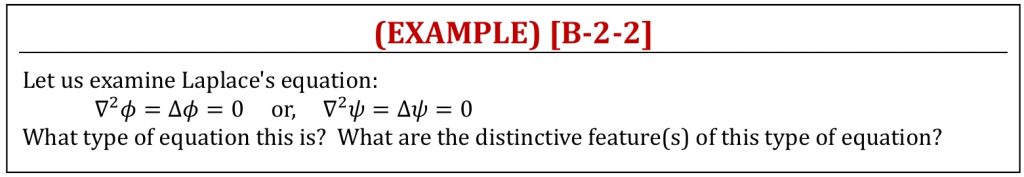
In conclusion, the Laplace’s equation is a linear 2nd order elliptic PDE.  The distinctive features include: (i) analytical solutions exist, with a given boundary conditions (called, the “elementary potential flow solutions“) and (ii) these elementary potential flow solutions can be “superimposed” to construct another valid solution of the flow field.  Laplace’s equation is the governing equation for an ideal flow field. Therefore, one can analyze flow field behavior (i.e., velocity, pressure, aerodynamic forces and moments) of an ideal flow field by mathematically solving the Laplace’s equation.  This is the very foundation of aerodynamics (theoretical aerodynamics).

References

• 2D & 3D Aerodynamics by P. Nathan (YouTube@PaulNathan82)
• The Efficient Engineer (https://efficientengineer.com)
• Fundamentals of Aerodynamics by J.D. Anderson, 5th ED, McGraw Hill, 2016
• Aerodynamics for Engineers by J. J. Bertin & M. L. Smith, 3rd ED, Cambridge University Press, 1997
• Aerodynamics for Engineering Students by E. L. Houghton & P. W. Carpenter, 4th ED, Edward Arnold, London, 1993

Media Attributions

If a citation and/or attribution to a media (images and/or videos) is not given, then it is originally created for this book by the author, and the media can be assumed to be under CC BY-NC 4.0 (Creative Commons Attribution-NonCommercial 4.0 International) license.  Public domain materials have been included in these attributions whenever possible.  Every reasonable effort has been made to ensure that the attributions are comprehensive, accurate, and up-to-date. The Copyright Disclaimer under Section 107 of the Copyright Act of 1976 states that allowance is made for purposes such as teaching, scholarship, and research.  Fair use is a use permitted by copyright statute.  For any request for corrections and/or updates, please contact the author.