A-2: Atmosphere
Altitude and Standard Atmosphere Model
Shigeo Hayashibara
What is Altitude?
Different Definitions for an “Altitude”
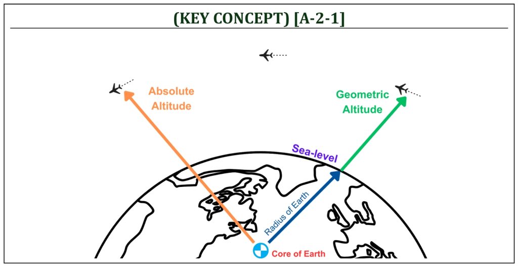
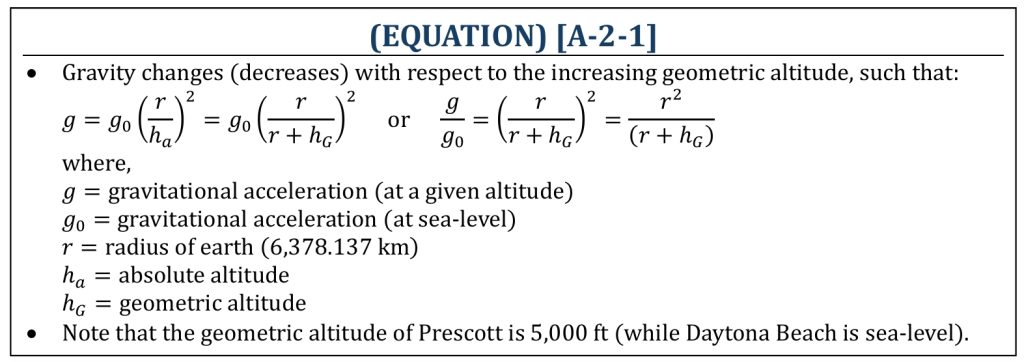
Unlike fluid mechanics, it is important to include the fact that the gravity being a variable with respect to the altitude in aerodynamics. When a standard model of of atmosphere (i.e., variation of temperature, pressure, and density) is constructed in aerodynamics, it is important to either include (or, like fluid mechanics, not to include to simplify the model) the fact that the gravity being a variable with respect to the altitude itself. This will become increasingly important at higher altitudes, where gravity can be significantly lower value than that of the value on the surface of the earth (called, the sea-level). The sea-level standard gravity can be defined as: 9.81 m/s2 or 32.2 ft/s2. To begin with, let’s identify two different definitions of an altitude in aerodynamics: (i) absolute altitude (ha): an altitude measured from the center of the earth and (ii) geometric altitude (hG): an altitude measured from the surface of the earth. Obviously, the gravitational acceleration is not constant: it will change (decrease), as the altitude becomes higher (departing away from the surface of the earth, i.e., from the center of the planet). Unlike fluid mechanics, it is desired in aerodynamics to include the effects of changing gravitational acceleration (with respect to altitude) into the standard atmospheric model for better accuracy (especially at higher altitudes). The variation of gravitational acceleration can be defined as a function of the earth radius and altitude.
Variation of Gravitational Acceleration
In order to incorporate the variation of the gravitational acceleration into a mathematical model of the earth’s atmosphere (called the standard atmosphere model), one needs to introduce a fictitious altitude (called, the geopotential altitude). The geopotential altitude (h) is not an actual physical altitude. It is a fictitious equivalent altitude against geometric altitude (hG), if (fictitiously) the gravitational acceleration is assumed to be a constant value (sea-level value: g0) throughout the atmosphere in entire altitude. This is necessary to perform all computations of atmospheric condition (i.e., variation of temperature, pressure, and density) under the non-constant gravitational acceleration (with respect to the altitude) of earth: g = g(h).
Hydrostatic Equation
Hydrostatic Equation for a Static Air
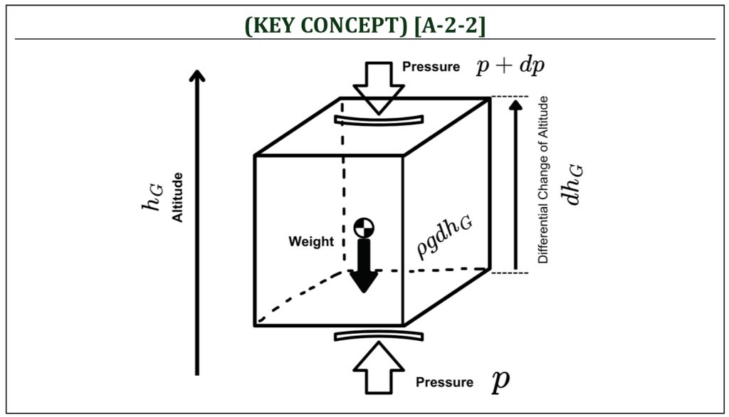
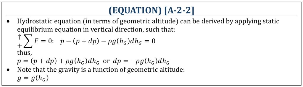
Let’s take a close look at a small cubic element of the air (atmosphere). If we apply the equation of equilibrium (statics) to this element in vertical direction (the direction of altitude), the governing equation (called the hydrostatic equation) can be derived, in terms of geometric altitude (hG).
Hydrostatic Equation in terms of geometric Altitude
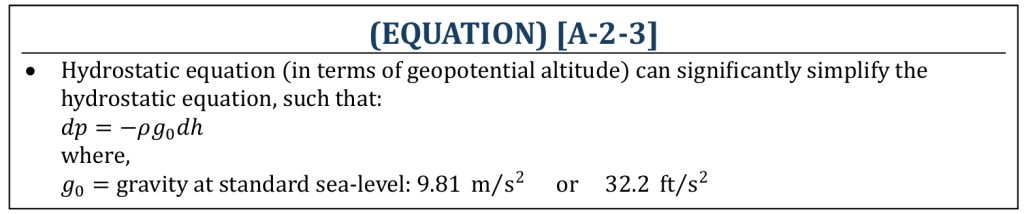
Note that, being the gravitational acceleration set to constant (g = g0), the geopotential altitude (h) will significantly simplify the mathematical model of the standard atmosphere.
Hydrostatic Equation in terms of geopotential Altitude
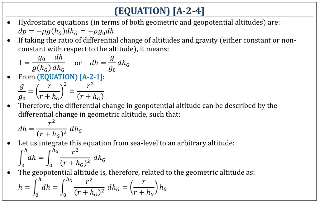
Note that the relationship between geometric (hG) and geopotential (h) altitudes must be clearly defined, however. The hydrostatic equation can be defined by both in terms of geometric (hG) and geopotential (h) altitudes.
Geopotential Altitude
The standard procedure of calculating the standard atmosphere can be summarized in the following 2 stages:
(i) A given geometric altitude (hG) must be converted to the corresponding geopotential altitude (h). The temperature variation within the atmosphere is given all based on geopotential altitude (h) starting from here. (ii) An appropriate set of equations (either for the gradient region or for the isothermal layer) need to be applied to calculate values of temperature (T), pressure (p), and density (ρ) at the given geopotential altitude (h), starting from the base altitude of either gradient region or isothermal layer.
The International Standard Atmosphere (ISA)
ISA Standard Temperature Variation Model
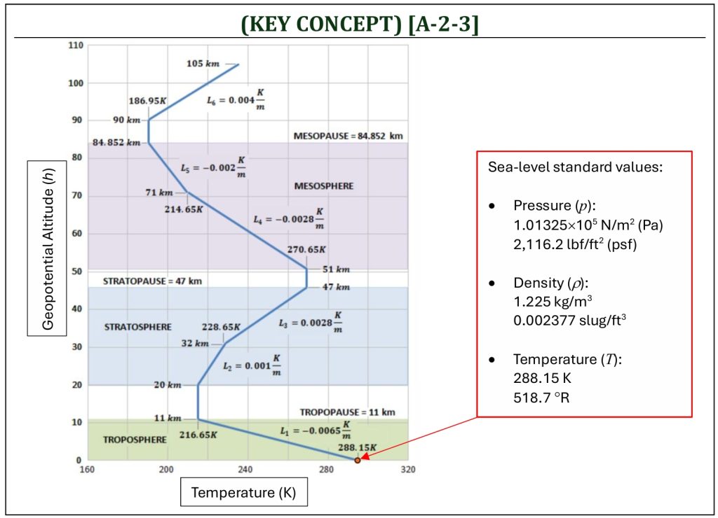
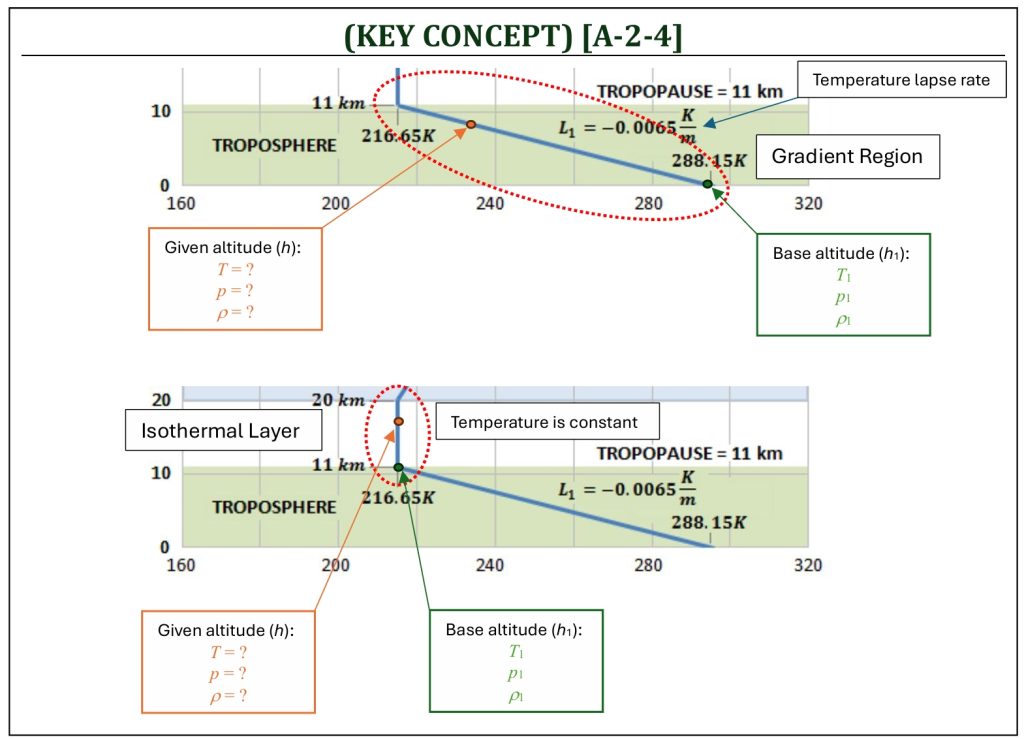
The baseline assumption of the standard atmosphere is the defined variation of temperature (T) with altitude, that is fairly consistent. It consists of a series of linearly varying temperature (called gradient regions) and constant temperature (called isothermal layers).
The first gradient region is called the troposphere, and the first isothermal layer is called the tropopause. Starting from the hydrostatic equation (with geopotential altitude), it is possible to construct a series of equations to calculate values of temperature (T), pressure (p), and density (ρ) at the given geopotential altitude (h).
The pressure variation within the standard atmosphere model can be obtained by the straight application of the hydrostatic equation.
Pressure Variation from Hydrostatic Equation
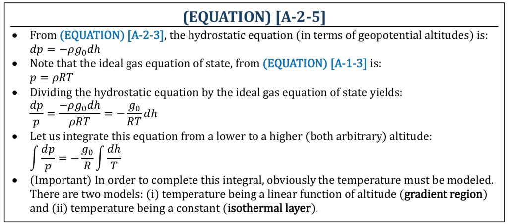
Now, in order to complete this integral, it is required to have the behavior of temperature with respect to the change of altitude. The following two different models (depending on the range of altitude) can be employed: (i) A range of altitude, where the temperature can be modeled as a linearly changing function (either linearly decreasing or increasing with a constant slope, a lapse rate; this is called a gradient region of atmosphere). (ii) A range of altitude, where the temperature can be assumed to be constant (this is called an isothermal layer of atmosphere).
Standard Atmosphere Model
Standard Atmosphere Model and Mathematical Calculations
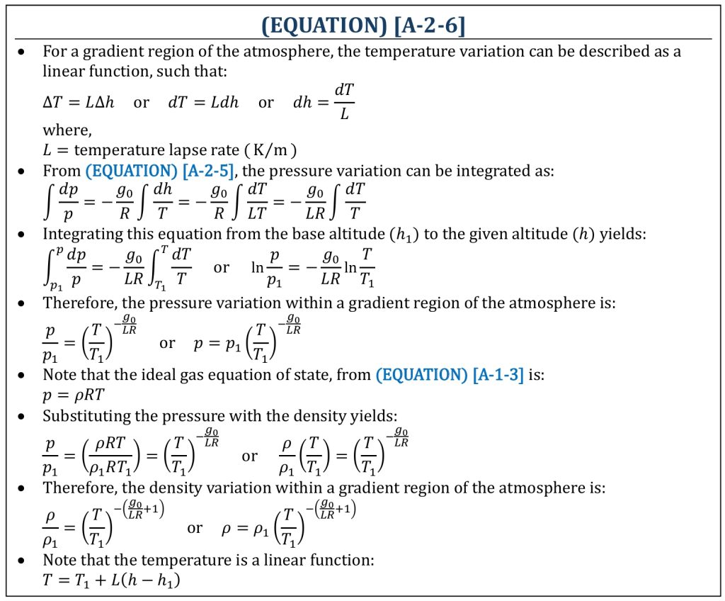
First, let us take a look at a gradient region. The temperature in this altitude range is assumed to be a linear function, either linearly increasing or decreasing with altitude. The hydrostatic equation can be integrated by treating the temperature as a linear function. The result will be a series of algebraic equations of temperature (T), pressure (p), and density (ρ).
Gradient Region Equations
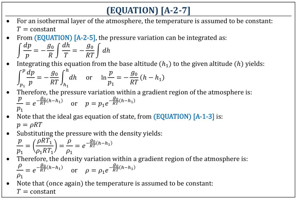
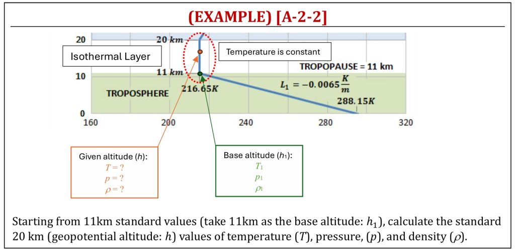
The second model is an isothermal layer. This is the layer where the temperature variation is assumed to be constant.
Isothermal Layer Equations
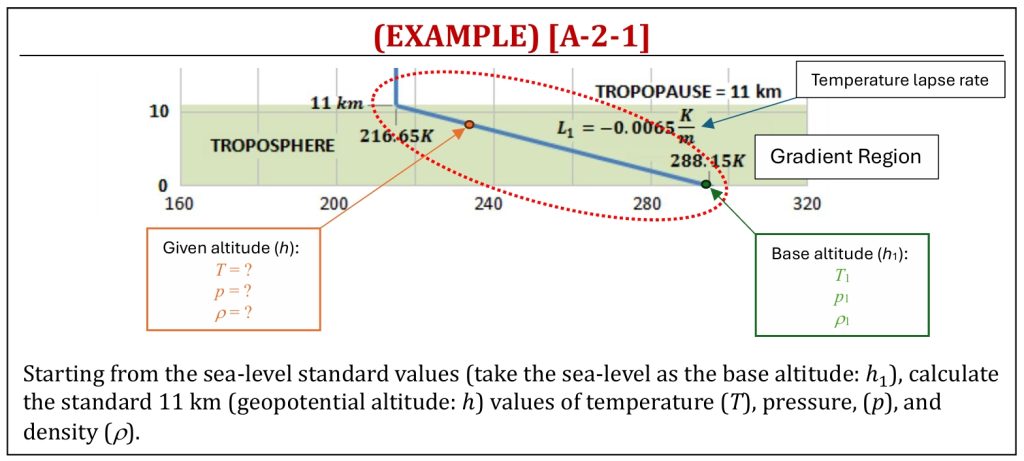
Gradient Region Computations (Troposphere)
Isothermal Layer Computations (Tropopause)
References
- Aerodynamics for Students by Auld & Srinivas (www.aerodynamics4students.com)
- Fundamentals of Aerodynamics by J.D. Anderson, 5th ED, McGraw Hill, 2016
- Aerodynamics for Engineers by J. J. Bertin & M. L. Smith, 3rd ED, Cambridge University Press, 1997
- Aerodynamics for Engineering Students by E. L. Houghton & P. W. Carpenter, 4th ED, Edward Arnold, London, 1993
Media Attributions
If a citation and/or attribution to a media (images and/or videos) is not given, then it is originally created for this book by the author, and the media can be assumed to be under CC BY-NC 4.0 (Creative Commons Attribution-NonCommercial 4.0 International) license. Public domain materials have been included in these attributions whenever possible. Every reasonable effort has been made to ensure that the attributions are comprehensive, accurate, and up-to-date. The Copyright Disclaimer under Section 107 of the Copyright Act of 1976 states that allowance is made for purposes such as teaching, scholarship, and research. Fair use is a use permitted by copyright statute. For any request for corrections and/or updates, please contact the author.