D-4: LLT and VLM for Finite Wings

Shigeo Hayashibara

D-4: LLT and VLM for Finite Wings

Prandtl's Classical Lifting Line Theory (LLT) and Numerical Vortex Lattice Method (VLM)

Shigeo Hayashibara

Vortex Filament

The Biot-Savart Law of a Vortex Filament

The Lifting Line Theory (LLT) and the lifting surface theory (often called: Vortex Lattice Method, or VLM), as well as 3-D panel method are all built upon potential flow analysis. In other words, these are pure theoretical schemes. As we deal with the pure theory, one must be aware (and keep track of) of the inherent assumptions within each theory-based method. All of these methods are developed under the assumptions to simplify the flow field physics:

Flow field is “steady state” (time independent).
Flow field is “inviscid” (viscosity, i.e., boundary layer, is ignored).
“No body force” (gravitational effect is ignored for the flow of “air”).
Flow field is “irrotational” ( $\nabla \times \overrightarrow{V} = \overrightarrow{0}$ ), and this will be able to define velocity potential ( $\phi$ ).
“Incompressible” flow (constant density, and this typically means “low subsonic” flow regime: $M_{\infty} < 0.3$ ).

Because of the assumptions made, the “pure theory” based results often does not accurately represent “real” flow field. It is crucial to recognize “what physics” were ignored and “what additional physical models” need to be added onto the solution. Typically, these “add-on” physical models include:

Compressibility corrections (for flows of: $M_{\infty} > 0.3$ ); note that flow field of high transonic to supersonic will become highly non-linear and a “correction” may become inaccurate.
Boundary layer models; note that the modeling of the surface boundary layer is typically an independent solution and added onto the base (inviscid) solution to represent the full solution with viscous effects included.

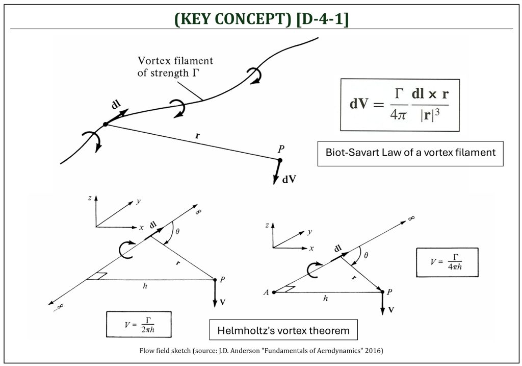
Let us recall mathematical concept of a vortex filament (defined as a straight line, made by a series of point vortices, in a certain direction). Technically, a vortex filament can also be curved, and the filament (with strength $\Gamma$ ) induces a flow field in the surrounding flow field.

A small velocity induced at an arbitrary location ( $P$ ) by a small segment ( $d\overrightarrow{l}$ ) of a given vortex filament (with strength: $\Gamma$ ) can be represented (note: this is called, the “Biot-Savart Law“), such that:

$d\overrightarrow{V} = \frac{\Gamma}{4\pi}\frac{d\overrightarrow{l} \times \overrightarrow{r}}{\left| \overrightarrow{r} \right|^{3}}$

Now, solving the Biot-Savart Law for a straight vortex filament of infinite (or semi-infinite) length will provide an important tool to represent basic behavior of an aircraft wing. This is know as the “Helmholtz’s Vortex Theorem.” Considering a straight vortex filament of infinite length, the velocity induced at an arbitrary point ( $P$ ) by the directed segment of a vortex filament ( $d\overrightarrow{l}$ ) is:

$V = \frac{\Gamma}{4\pi}\int_{- \infty}^{+ \infty}{\frac{\sin(\theta)}{r^{2}}dl}$

Let $h$ be the perpendicular distance from point $P$ to the vortex filament, such that:

$r = \frac{h}{\sin(\theta)}\ \ \ \ \text{and}\ \ \ \ \ l = \frac{h}{\tan(\theta)}$

Then,

$dl = - \frac{h}{\sin^{2}(\theta)}d\theta$

Therefore, the induced velocity is:

$V = \frac{\Gamma}{4\pi}\int_{- \infty}^{+ \infty}{\frac{\sin(\theta)}{r^{2}}dl} = - \frac{\Gamma}{4\pi}\int_{\pi}^{0}{\sin(\theta)d\theta} = \frac{\Gamma}{2\pi h}$

In case of a semi-infinite straight vortex filament,

$V = \frac{\Gamma}{4\pi h}$

Lifting Line Theory

Horseshoe Vortex and Downwash

KEY CONCEPT [D-4-2]

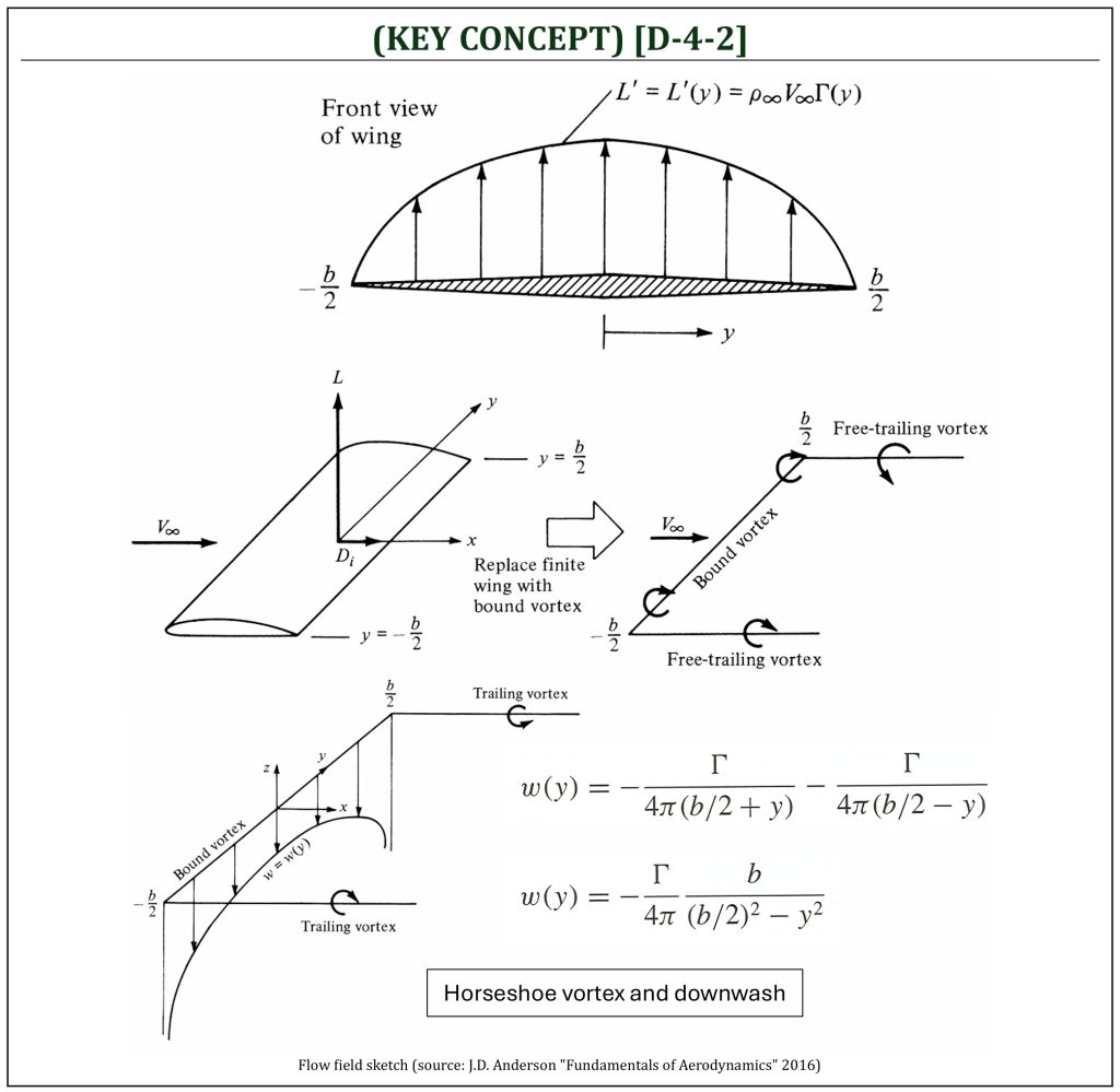
The basic idea of Prandtl’s classic lifting line theory is to represent a finite (3-D) wing using a vortex filament. A simple vortex filament of strength $\Gamma$ that is bound to a fixed location in a flow (this is called, the “bound vortex“) will generate a lift force (per unit span): $L^{'} = \rho_{\infty}V_{\infty}\Gamma$ (from the Kutta-Joukowski theorem). A finite wing can be replaced with a bound vortex, which extends from wingtip ( $y = - \frac{b}{2}$ ) to wingtip ( $y = + \frac{b}{2}$ ) with two free-trailing edge vortices (called, the “horseshoe” vortex).

If the origin of this horseshoe vortex is taken at the center of the bound vortex, two semi-infinite vortex filaments induce the velocity (called, the “downwash”):

$w(y) = - \frac{\Gamma}{4\pi\left( \frac{b}{2} + y \right)} - \frac{\Gamma}{4\pi\left( \frac{b}{2} - y \right)} = - \frac{\Gamma}{4\pi}\frac{b}{\left( \frac{b}{2} \right)^{2} - y^{2}}$

However, the downwash distribution, due to the single horseshoe vortex, does not realistically simulate that of a finite wing. Instead of representing the wing by a single horseshoe vortex, let us superimpose a large number of horseshoe vortices, each with a different length of the bound vortex, but with all the bound vortices coincide along a single line (this is called, the “lifting line“).

Prandtl’s Lifting Line Theory (LLT)

KEY CONCEPT [D-4-3]

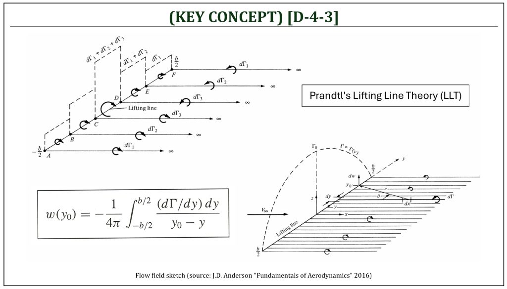
An infinite number of horseshoe vortices superimposed along the lifting line will produce a desired distribution of vortex strength, $\Gamma = \Gamma(y)$ , along the lifting line. At an arbitrary spanwise location ( $y_{0}$ ), a differential downward velocity (downwash) $dw$ is induced as:

$dw = - \frac{\left( \frac{d\Gamma}{dy} \right)dy}{4\pi\left( y_{0} - y \right)}$

Then, the downwash induced at this location ( $y_{0}$ ) is:

$w\left( y_{0} \right) = - \frac{1}{4\pi}\int_{- \frac{b}{2}}^{\frac{b}{2}}\frac{\left( \frac{d\Gamma}{dy} \right)dy}{y_{0} - y}$

The induced angle of attack due to downwash at this location ( $y_{0}$ ) is:

$\alpha_{i}\left( y_{0} \right) = \tan^{- 1}\left\lbrack \frac{- w\left( y_{0} \right)}{V_{\infty}} \right\rbrack\ \ \ \$

Assuming a small angle, $\tan^{- 1}(\theta) \approx \theta$ , the induced angle of attack is:

$\alpha_{i}\left( y_{0} \right) = \frac{- w\left( y_{0} \right)}{V_{\infty}}$

In conclusion, the induced angle of attack can be calculated as:

$\alpha_{i}\left( y_{0} \right) = \frac{1}{4\pi V_{\infty}}\int_{- \frac{b}{2}}^{\frac{b}{2}}\frac{\left( \frac{d\Gamma}{dy} \right)dy}{y_{0} - y}$

The effective angle of attack ( $\alpha_{\text{eff}}$ ) is the angle of attack actually seen by the local airfoil section, that is: $\alpha_{\text{eff}} = \alpha_{\text{eff}}\left( y_{0} \right)$ . Note that: $\alpha_{\text{eff}} = \alpha - \alpha_{i}$ , then the section lift coefficient can be found as:

$c_{l}\left( y_{0} \right) = \alpha_{0}\left\lbrack \alpha_{\text{eff}}\left( y_{0} \right) - \alpha_{L = 0}\left( y_{0} \right) \right\rbrack = 2\pi\left\lbrack \alpha_{\text{eff}}\left( y_{0} \right) - \alpha_{L = 0}\left( y_{0} \right) \right\rbrack$

From Kutta-Joukowski theorem, the lift force (per unit span) can be computed:

$L^{'} = 0.5\rho_{\infty}V_{\infty}^{2}c\left( y_{0} \right)c_{l} = \rho_{\infty}V_{\infty}\Gamma\ \ \ \ \text{or}\ \ \ \ \ c_{l}\left( y_{0} \right) = \frac{2\Gamma\left( y_{0} \right)}{V_{\infty}c\left( y_{0} \right)}$

Hence, the lift coefficient can be expressed as:

$c_{l}\left( y_{0} \right) = \frac{2\Gamma\left( y_{0} \right)}{V_{\infty}c\left( y_{0} \right)} = 2\pi\left\lbrack \alpha_{\text{eff}}\left( y_{0} \right) - \alpha_{L = 0}\left( y_{0} \right) \right\rbrack$

Solving this equation for the effective angle of attack yields:

$\alpha_{\text{eff}}\left( y_{0} \right) = \frac{\Gamma\left( y_{0} \right)}{\pi V_{\infty}c\left( y_{0} \right)} + \alpha_{L = 0}\left( y_{0} \right)$

Also, note that: $\alpha_{\text{eff}} = \alpha - \alpha_{i}\ \text{thus} \ \alpha = \alpha_{\text{eff}} + \alpha_{i}$ ; therefore, the angle of attack can be expressed as:

$\alpha\left( y_{0} \right) = \frac{\Gamma\left( y_{0} \right)}{\pi V_{\infty}c\left( y_{0} \right)} + \alpha_{L = 0}\left( y_{0} \right) + \frac{1}{4\pi V_{\infty}}\int_{- \frac{b}{2}}^{\frac{b}{2}}\frac{\left( \frac{d\Gamma}{dy} \right)dy}{y_{0} - y}$

Lifting Line Theory for a straight wing

Simple Lifting Line Theory (LLT) Example

KEY CONCEPT [D-4-4]

In summary, the lifting line theory solutions for a finite wing can be summarized into the following step-by-step analytical process:

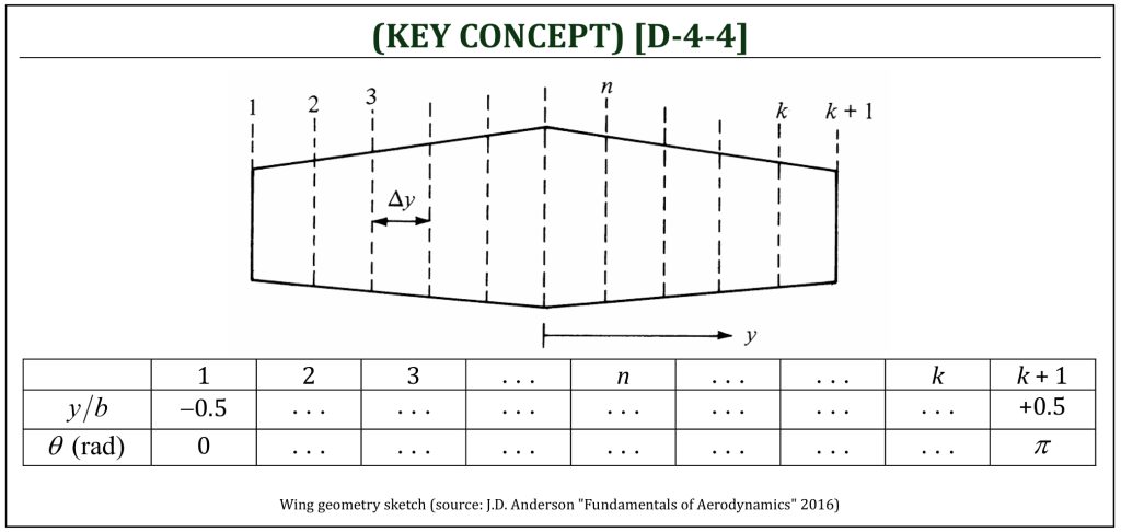
(1) Divide the wing into a number of spanwise stations: for example, stations as shown in the figure, with designating any specific spanwise station.

where, coordinate transformation ( $y \rightarrow \theta$ ) is:

$y = - \frac{b}{2}\cos(\theta)\ \ \ \ \text{and}\ \ \ \ \theta = \cos^{- 1}\left( - \frac{2}{b}y \right)$

(2) Calculate wing geometric parameters:

Aspect ratio:

$AR = \frac{b}{c_{\text{avg}}} = \frac{b^{2}}{S} = \frac{2b}{c_{r}(1 + \lambda)}\ \ \ \ \text{Note that: }\lambda \text{(taper ratio)} = \frac{c_{t} \text{(tip\ chord)}}{c_{r} \text{(root\ chord)}}$

Average chord length:

$c_{\text{avg}} = \frac{\left( c_{r} + c_{t} \right)}{2} = \frac{c_{r}(1 + \lambda)}{2}$

Wing (planform) area:

$S = c_{\text{avg}} \cdot b = \frac{\left( c_{r} + c_{t} \right)b}{2} = \frac{c_{r}(1 + \lambda)b}{2}$

(3) Determine the chord length at a given spanwise station ( $c(y))$ , which is given by:

$c(y) = c_{r}\left\lbrack 1 + (1 - \lambda)\frac{2y}{b} \right\rbrack\ \left( - \frac{b}{2} \leq y \leq 0 \right)$

and

$c(y) = c_{r}\left\lbrack 1 - (1 - \lambda)\frac{2y}{b} \right\rbrack\ \left( 0 \leq y \leq \frac{b}{2} \right)$

or, in terms of $\theta$ :

$c(\theta) = c_{r}\left\lbrack 1 + (\lambda - 1)\cos(\theta) \right\rbrack\ \left( 0 \leq \theta \leq \frac{\pi}{2} \right)$

and

$c(\theta) = c_{r}\left\lbrack 1 - (\lambda - 1)\cos(\theta) \right\rbrack\ \left( \frac{\pi}{2} \leq \theta \leq \pi \right)$

(4) Apply the Prandtl’s lifting line equations along the defined lifting line:

$\alpha = \frac{AR(1 + \lambda)}{\pi\left\lbrack 1 + (\lambda - 1)\cos(\theta) \right\rbrack}\sum_{n = 1}^{N}{A_{n}\sin(n\theta)} + \sum_{n = 1}^{N}{{nA}_{n}\frac{\sin(n\theta)}{\sin(\theta)}}\ \left( 0 \leq \theta \leq \frac{\pi}{2} \right)$

$\alpha = \frac{AR(1 + \lambda)}{\pi\left\lbrack 1 - (\lambda - 1)\cos(\theta) \right\rbrack}\sum_{n = 1}^{N}{A_{n}\sin(n\theta)} + \sum_{n = 1}^{N}{{nA}_{n}\frac{\sin(n\theta)}{\sin(\theta)}}\ \left( \frac{\pi}{2} \leq \theta \leq \pi \right)$

(5) Solve coefficients (simultaneous $n$ equations with $n$ unknowns):

$A_{1},\ \ A_{2},\ \ A_{3},\ .\ \ .\ \ .\ ,\ A_{n}$

(6) Calculate aerodynamic coefficients:

The lift coefficient of the wing:

$C_{L} = \pi(AR)\left( A_{1} \right)$

The induced drag coefficient of the wing:

$C_{D,i} = \pi(AR)\sum_{n = 1}^{N}{nA_{n}^{2}}$

Span efficiency factor of the wing:

$e = \frac{C_{L}^{2}}{\pi(AR)\left( C_{D,i} \right)}$

(7) Calculate the section lift coefficient distribution:

$c_{l} = \frac{4b}{c}\sum_{n = 1}^{N}{A_{n}\sin(n\theta)}$

or, in terms of $\theta$ :

$c_{l} = \frac{2(AR)(1 + \lambda)}{1 + (\lambda - 1)\cos(\theta)}\sum_{n = 1}^{N}{A_{n}\sin(n\theta)}\ \left( 0 \leq \theta \leq \frac{\pi}{2} \right)$

$c_{l} = \frac{2(AR)(1 + \lambda)}{1 - (\lambda - 1)\cos(\theta)}\sum_{n = 1}^{N}{A_{n}\sin(n\theta)}\ \left( \frac{\pi}{2} \leq \theta \leq \pi \right)$

(8) Calculate the section lift distribution (normalized lift distribution):

$\frac{c(y)c_{l}(y)}{c_{\text{avg}}C_{L}} = \frac{4(AR)}{C_{L}}\sum_{n = 1}^{N}{A_{n}\sin(n\theta)}\ (0 \leq \theta \leq \pi)$

For the case of elliptical spanwise lift distribution (ideal case, span efficiency e = 1):

$\frac{c(y)c_{l}(y)}{c_{\text{avg}}C_{L}} = \frac{4(AR)}{C_{L}}A_{1}\sin(\theta)\ (0 \leq \theta \leq \pi)$

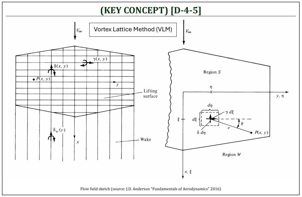
Lifting surface (Vortex LatTice) method

Vortex Lattice Method (VLM)

KEY CONCEPT [D-4-5]

Prandtl’s Lifting Line Theory (LLT) predicts finite wing lift in a wide range of angle of attack fairly well. The wing lift coefficient ( $C_{L}$ ) v.s. angle of attack ( $\alpha$ ) prediction is fairly accurate in pre-stall condition, as well as “post-stall” (high angle of attack) conditions (typically within 20% error range) compared against experimental results. The LLT method provides fairly reasonable preliminary engineering results for the high angle of attack post-stall conditions. Prandtl’s Lifting Line Theory (LLT) offers fairly reasonable results for straight wings with moderate to high aspect ratio. However, the theory is not applicable for low aspect ratio straight wings, swept wings, and delta wings.

Prandtl’s Lifting Line Theory (LLT) can be extended to a more robust and flexible method by application of today’s high-performance computing capability. Essentially, a surface of a body (could be a wing, fuselage, or any surface of a vehicle) can be represented by a small “lattice” area with corresponding superimposed horseshoe vortex (similar to the lifting line). This is the “lifting surface” method, often called the “Vortex Lattice Method” (VLM).

Extending the model by placing a series of lifting lines on the plane of the wing, at different chordwise stations; that is to consider a large number of lifting lines all parallel to the spanwise ( $y$ ) location, located at different values of chordwise ( $x$ ) location.

The lifting surface is defined by the following two parameters:

(i) horizontal vortex sheet of strength: $\gamma = \gamma(x,y)$

(ii) vertical vortex sheet of strength: $\delta = \delta(x,y)$

From the Biot-Savart law, the incremental velocity ( $\ |d\overrightarrow{V}|$ ) induced at point $P$ by a small segment ( $d\eta$ ) of this vortex filament of strength ( $\gamma d\xi$ ) is:

$\ |d\overrightarrow{V}|=\left| \frac{\Gamma}{4\pi}\frac{d\overrightarrow{l}\times \overrightarrow{r}}{\left| \overrightarrow{r} \right|^3} \right| = \frac{\gamma d\xi}{4\pi}\frac{(d\eta)r\sin(\theta)}{r^{3}}$

Considering the contribution of the elemental spanwise vortex of strength ( $\gamma d\xi$ ) to the induced velocity at point $P$ :

$(dw)_{\gamma} = - \frac{\gamma}{4\pi}\frac{(x - \xi)d\xi d\eta}{r^{3}}$

Considering the contribution of the elemental chordwise vortex of strength ( $\delta d\eta$ ) to the induced velocity at point $P$ :

$(dw)_{\delta} = - \frac{\delta}{4\pi}\frac{(y - \eta)d\xi d\eta}{r^{3}}$

Note that:

$r = \sqrt{(x - \xi)^{2} + (y - \eta)^{2}}$

To obtain the velocity induced at point $P$ by the entire lifting surface, these equations must be integrated over the wing planform, designated as region $S$ . Moreover, the velocity induced at point $P$ by the complete wake needs to be considered ( $\delta_{w}$ instead of $\delta$ ) in the wake region.

Therefore, the induced velocity (induced at point $P$ ) by both the lifting surface and the wake can be expressed in the following equation:

$w(x,y) = - \frac{1}{4\pi}\iint_{S}^{\ }{\frac{(x - \xi)\gamma(\xi,\eta) + (y - \eta)\delta(\xi,\eta)}{\left\lbrack (x - \xi)^{2} + (y - \eta)^{2} \right\rbrack^{\frac{3}{2}}}d\xi d\eta}$

$- \frac{1}{4\pi}\iint_{S}^{\ }{\frac{(y - \eta)\delta_{w}(\xi,\eta)}{\left\lbrack (x - \xi)^{2} + (y - \eta)^{2} \right\rbrack^{\frac{3}{2}}}d\xi d\eta}$

The central problem of lifting-surface theory (i.e., VLM) is to solve this equation for $\gamma(\xi,\eta)$ and $\delta(\xi,\eta)$ such that the sum of the induced velocity $w(x,y)$ and the normal component of the freestream velocity become zero on every lifting surface of the body. This is called the “flow tangency” condition of the lifting surface (means that the body surface can be represented by series of stagnation streamlines), which is essentially the very similar fundamental concept of thin airfoil theory or 2-D (or 3-D) panel method.

References

Aerodynamics for Students by Auld & Srinivas (www.aerodynamics4students.com)
Fundamentals of Aerodynamics by J.D. Anderson, 5th ED, McGraw Hill, 2016
Aerodynamics for Engineers by J. J. Bertin & M. L. Smith, 3rd ED, Cambridge University Press, 1997
Aerodynamics for Engineering Students by E. L. Houghton & P. W. Carpenter, 4th ED, Edward Arnold, London, 1993

Software

The software application is available (from www.aerodynamics4students.com) to simulate flow field of wings (LLT: without wing sweep). The program assumes a linear variation of section properties between wing root and tip. The wing loading is assumed to be symmetric about the wing root. Section lift data in terms of $a_{0}$ , $\alpha_{L=0}$ is required for the wing root and the wing tip sections, such that:

$c_{l}(\text{2-D}) = a_{0}\left( \alpha_{\text{2-D}} - \alpha_{L=0} \right)$

This can be obtained from published 2-D experimental data or theoretical techniques such as thin airfoil theory (C-3).

The program uses the lifting line equations to get solutions for lift coefficient versus angle of attack and induced drag coefficient versus square of the lift coefficient. For a given angle of attack, the program will display the resulting distribution of section lift coefficient across the span, the distribution of downwash at the wing and a listing of the solution Fourier coefficients for this angle. A flapped section (control surfaces) can also be specified in the input. The percentage of wing span with flap must be defined to create a flapped wing section. The flap section properties are assumed to be those entered for the wing root section. These section properties will be kept constant across the flapped portion of the span for simplification. The section properties used outboard of the flap will also be constant and assumed to be equal to those of the wing tip for simplification.

3-D Finite (Straight Tapered) Wing: Prandtl’s Lifting Line Theory (LLT) Solver

The software application is available (from aerodynamics4students.com) to simulate flow field of wings (VLM: including wing sweep). The program assumes a linear variation of planform for up to two zones and a simple planar tailplane. Zone 1 covers wing root to specified span location, then Zone 2 covers span location to wing tip. The section properties can vary linearly across each zone between wing root, mid-span and tip or a constant section can be set for each zone.

The entire wing geometry is assumed to be symmetric about the wing root. The tailplane can be set at a required distance behind the wing root with a constant chord and sweep angle. A center of gravity (“CG“) location (in terms of the fraction of root chord behind leading edge) can be set, so that calculated $C_{m}$ coefficients will be relative to this point. The airfoil section properties for the wing root, mid-span and tip can be specified by entering a chord length and zero lift angle. This will generate a mean line for each section which corresponds to the input section properties. An incidence angle can also be set for the tail.

VLM Geometry

EXAMPLE [D-4-1]

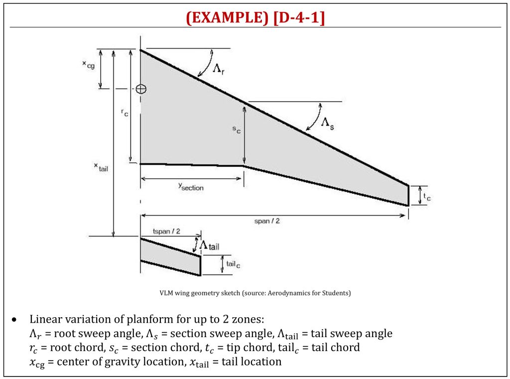
The origin is at wing root leading edge and the center of gravity (“CG“) location is defined as a fraction of the root chord from leading edge. The program uses the vortex lattice method equations to obtain solutions for lift coefficient versus angle of attack, pitching moment coefficient versus angle and induced drag coefficient versus square of the lift coefficient. For a given angle of attack the program will display the resulting differential pressure coefficient distribution.

3-D Finite Wing: Vortex Lattice Method (VLM) Solver

Media Attributions

If a citation and/or attribution to a media (images and/or videos) is not given, then it is originally created for this book by the author, and the media can be assumed to be under CC BY-NC 4.0 (Creative Commons Attribution-NonCommercial 4.0 International) license. Public domain materials have been included in these attributions whenever possible. Every reasonable effort has been made to ensure that the attributions are comprehensive, accurate, and up-to-date. The Copyright Disclaimer under Section 107 of the Copyright Act of 1976 states that allowance is made for purposes such as teaching, scholarship, and research. Fair use is a use permitted by copyright statute. For any request for corrections and/or updates, please contact the author.

License

Icon for the Creative Commons Attribution-NonCommercial 4.0 International License