C-3: Thin Airfoil Theory

Shigeo Hayashibara

C-3: Thin Airfoil Theory

Pradtl's Classical 2-D Symmetric and Cambered Thin Airfoil Theory

Shigeo Hayashibara

A point vortex to a vortex panel

Vortex Panel

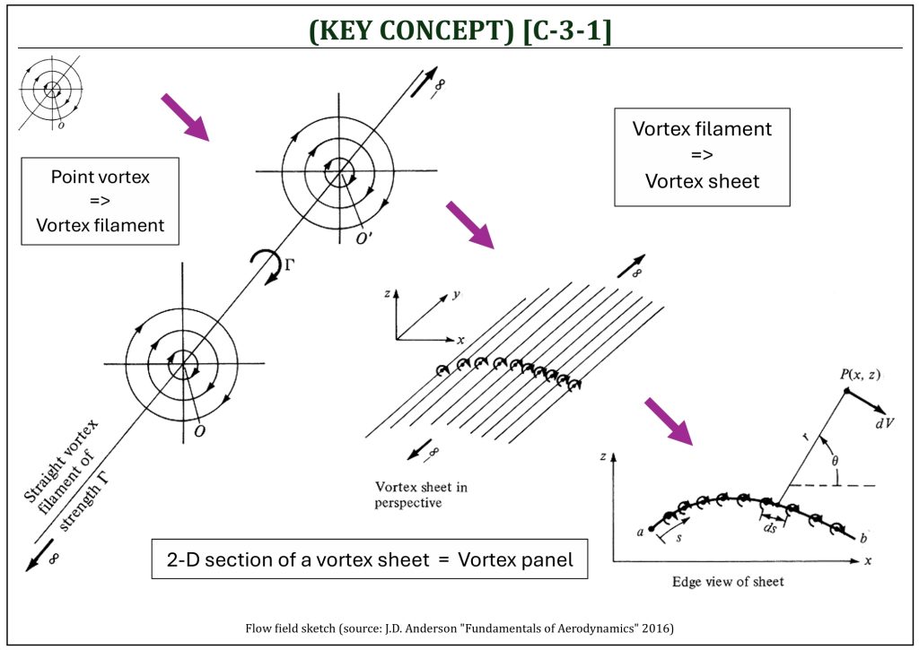
At this moment, let us review KEY CONCEPT [B-3-7] once again. Based on the potential flow analysis (pure mathematical analysis), a point vortex of strength $\Gamma$ will create the corresponding solution in terms of either velocity potential or stream function, such that:

$\phi = - \frac{\Gamma}{2\pi}\theta\ \ \ \ \text{or,}\ \ \ \ \psi = \frac{\Gamma}{2\pi}\ln r$

Employing the stream function ( $\psi$ ), the velocity field induced by the presence of this point vortex can be found as:

$V_{r} = \frac{1}{r}\frac{\partial\psi}{\partial\theta} = 0\ \ \ \ \text{and}\ \ \ \ \ V_{\theta} = - \frac{\partial\psi}{\partial r} = - \frac{\Gamma}{2\pi r}$

Note that the velocity field in 2-D polar coordinate system is represented by:

$\overrightarrow{V} = V_{r}{\widehat{e}}_{r} + V_{\theta}{\widehat{e}}_{\theta}$

The strength of a point vortex is the flow field “circulation,” and can be defined as:

$\Gamma = - \oint_{c}^{\ }{\overrightarrow{V} \cdot d\overrightarrow{s}} = - \oint_{0}^{2\pi}\left( V_{\theta}{\widehat{e}}_{\theta} \right) \cdot \left( rd\theta{\widehat{e}}_{\theta} \right) = - (2\pi r)V_{\theta}$

By simply extending this 2-D mathematical model of point vortex solution of Laplace’s equation, a 3-D “vortex filament” can be defined as a straight line, made by a series of point vortices, in a certain direction. This is a filament made by a series of point vortices. A typical vortex filament can be modeled as a straight line going through the series of point O, the origin of each vortex, extending to infinity on both sides of the filament. Now, one more step further, we can define a “vortex sheet.” A vortex sheet can be defined as a physical 3-D surface defined by a series of infinite number of vortex filaments, placed side by side, with the strength of each filament being infinitesimally small. The 2-D section of this vortex sheet is now defined as “vortex panel.” A vortex panel is a straight edge-line (a panel) generated by connecting neighboring vortex sheet with a straight line. It is now possible to use this vortex panel to numerically simulate a physical 2-D airfoil shape placed within a uniform flow field.

It is necessary to define the strength of a vortex panel, the circulation ( $\Gamma$ ), as a “circulation per unit length” ( $\gamma$ ) of each panel. Note that the circulation per unit length can be a variable, along the mean camber line (that means: $\gamma = \gamma(s)$ ). This will be depending on the strength (i.e., circulation) of each panel along the mean camber line, as a geometry is constructed as a series of short segments of straight edge-lines (i.e., panels). As obviously in nature, the thin airfoil theory is only an “approximation” of curved mean camber geometry with a series of short straight-edge lines (i.e., panels). Typically, the strength of each panel is set to uniform, but this can also be a variable within each panel (if so, this is called a higher-order thin airfoil method).

The flow field circulation is induced by each panel by:

$\gamma = \gamma(s)$

and, therefore:

$d\Gamma = \gamma ds$

Consider an arbitrary point $P(x,z)$ in a simulated potential flow field. A small section of vortex panel of strength $\gamma ds$ induces a small velocity potential (as well as the velocity) in the flow field:

$d\phi = - \frac{\Gamma}{2\pi}\theta = - \frac{\gamma ds}{2\pi}\theta\ \ \ \ \text{and}\ \ \ \ dV = - \frac{\gamma ds}{2\pi r}$

The velocity potential and the circulation induced, at point $P(x,z)$ due to the entire vortex sheet, representing the mean camber line of a flat plate airfoil can be found by integration (from the leading edge to the trailing edge) of the given sheet, representing the mean camber line of a flat plate airfoil, such that:

$\phi(x,z) = - \frac{1}{2\pi}\int_{a}^{b}{\theta\ \gamma ds}$

where, the flow field circulation can be defined by:

$\Gamma = \int_{a}^{b}{\gamma ds}$

Thin Airfoil Theory and Panel Method

KEY CONCEPT [C-3-2]

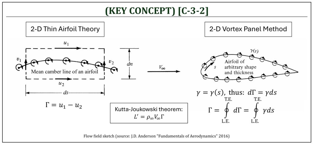
A series of vortex panels can be used to represent variety of shapes. If a mean camber line is represented (either as a “flat plate” or a “curved flat plate“), it is called the thin airfoil theory (“thin” means that the airfoil thickness is completely ignored). If the actual shape of a 2-D airfoil, with both upper and lower surfaces, is represented (either as a “symmetric airfoil” or “cambered airfoil“), it is called the panel method analysis (the actual shape, certainly including the airfoil thickness, is to be simulated).

Let’s consider a simple control volume analysis (dashed path) enclosing a vortex sheet with strength ( $\gamma ds$ ):

$\Gamma = - \oint_{c}^{\ }{\overrightarrow{V} \cdot d\overrightarrow{s}} = - \left( v_{2}dn - u_{1}ds - v_{1}dn + u_{2}ds \right)$

$= \left( u_{1} - u_{2} \right)ds + \left( v_{1} - v_{2} \right)dn$

where, $s$ is the tangential direction, and $n$ is the normal direction coordinates of the flow field.

Let both top and bottom control surfaces moving closer and closer to the vortex sheet (means that: $dn \rightarrow 0$ ), then the flow field circulation can be simply defined by:

$\Gamma = u_{1} - u_{2}$

This concludes that the local jump in tangential velocity across the vortex sheet is equal to the flow field circulation, and the flow field circulation can determine the lift (per unit depth) of this simulated 2-D flow field by Kutta-Joukowski theorem:

$Lift = \rho_{\infty}V_{\infty}\Gamma$

This is the fundamental concept of the thin airfoil theory. As this is essentially a flat plate (either straight flat plate = thin symmetric airfoil -or- bent flat plate = cambered thin airfoil). The Kutta condition (flow must have a smooth departure at the trailing edge) is naturally satisfied in thin airfoil theory by constraining the last panel to form the leading edge is equal to zero vortex strength ( $\gamma_{T.E.} = 0$ ).

Thin airfoil theory can only represent the mean camber line (airfoil thickness is essentially neglected); however, this thin airfoil theory can be further extended. It is certainly possible to use vortex panels to represent the complete surface shape (rather than just mean camber line) of a given airfoil. It is, actually, safe to say that the 2-D thin airfoil theory is a “simplified” version of the 2-D vortex panel method to simulate the flow field of an airfoil.

prandtl’s thin airfoil theory

Prandtl’s Classical Approach for Thin Airfoil Theory

KEY CONCEPT [C-3-3]

Thin airfoil theory is a simplified mathematical analysis of either symmetric or cambered “flat plate” airfoil. The mathematical solution of “Joukowski flat plate” airfoil (B-5) is essentially identical to the symmetric thin airfoil analysis solution. The cambered thin airfoil analysis solution will simulate the mean camber line of an airfoil, simply ignoring its thickness (hence, essentially it simulates a curved flat plate).

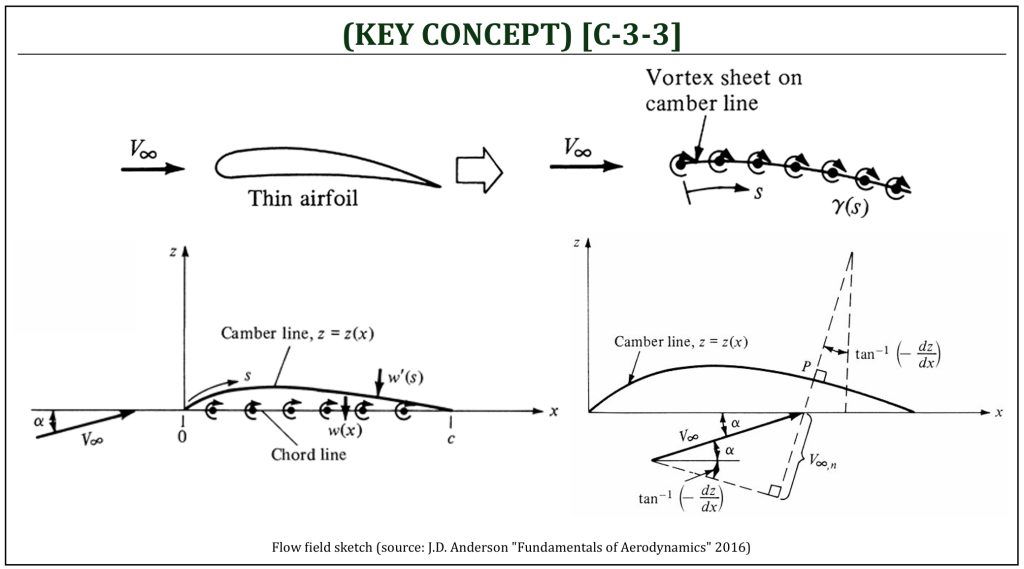
If the airfoil is very thin (ideally, a flat plate), a single vortex sheet can be used to approximate a thin airfoil by replacing it along the camber line. This is the basic concept of the thin airfoil theory. There are a few variations of thin airfoil theory, the classical Prandtl’s classical thin airfoil theory will be discussed here in details, based on the following simplification assumptions:

Rather than modeling the mean camber line itself by a vortex sheet, the chord line (means: the straight line connecting between leading edge and trailing edge) is represented by a vortex sheet as a function of straight horizontal coordinate system (x). Therefore, the vortex sheet is placed on the chord line: $\gamma = \gamma(x)$

The camber line is forced to be a streamline, and is calculated to satisfy this condition as well as Kutta condition (circulation at the trailing edge is zero, allowing the flow from both upper and lower surfaces depart smoothly): $\gamma(c) = 0$

For the camber line to be a streamline, the normal component of freestream ( $V_{\infty,n}$ ) is going to be cancelled by the downwash generated by the vortex sheet (everywhere along the mean camber line), $w^{'}(s)$ ; mathematically represented as: $V_{\infty,n} + w^{'}(s) = 0$

At an arbitrary point ( $P$ ) on the camber line, where the slope of the camber line can be defined, the normal component of freestream ( $V_{\infty,n}$ ) can be determined, such that:

$V_{\infty,n} = V_{\infty}\sin\left\lbrack \alpha + \tan^{- 1}\left( - \frac{dz}{dx} \right) \right\rbrack$

Note that for a thin airfoil, the following simplifications (“small angle approximations“) can be made:

$\sin{(\theta) \approx \tan{(\theta) \approx \theta}}$

Therefore, it can be simplified as:

$\sin{(\alpha) \approx \alpha$

and

$\tan^{- 1}\left( - \frac{dz}{dx} \right)\) \approx - \frac{dz}{dx}$

Therefore, it can be simplified as:

$V_{\infty,n} = V_{\infty}\left\lbrack \alpha - \left( \frac{dz}{dx} \right) \right\rbrack$

Induced Velocity from an Element (a Panel) of Vortex

KEY CONCEPT [C-3-4]

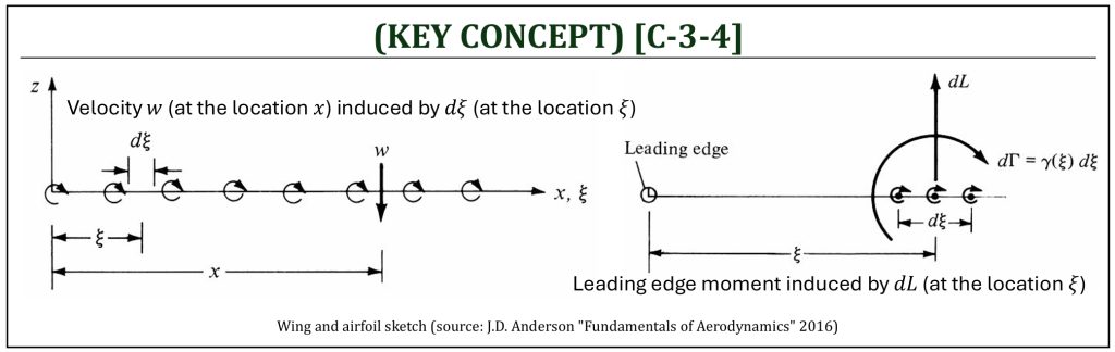
The velocity ( $dw$ ) at location $x$ induced by the small elemental vortex ( $d\xi$ ) at location $\xi$ can be described as:

$dw = - \frac{\gamma(\xi)d\xi}{2\pi(x - \xi)}$

Thus, the velocity $w(x)$ induced at location $x$ by all the elemental vortices along the chord line can be obtained by integrating $dw$ from the leading edge ( $\xi = 0$ ) to the trailing edge ( $\xi = c$ ) as:

$w(x) = - \int_{0}^{c}\frac{\gamma(\xi)d\xi}{2\pi(x - \xi)}$

For the camber to be a streamline, the condition ( $V_{\infty,n} + w^{'}(s) = 0$ ) must be satisfied. For the Prandtl’s classical thin airfoil theory, $w^{'}(s) \approx w(x)$ , as vortex sheet is placed on the chord line (rather than mean camber line) with an approximation of small angles; therefore,

$V_{\infty}\left( \alpha - \frac{dz}{dx} \right) - \int_{0}^{c}\frac{\gamma(\xi)d\xi}{2\pi(x - \xi)} = 0$

In conclusion, the governing equation of the Prandtl’s classical thin airfoil theory can be defined as:

$\frac{1}{2\pi}\int_{0}^{c}\frac{\gamma(\xi)d\xi}{x - \xi} = V_{\infty}\left( \alpha - \frac{dz}{dx} \right)$

symmetric thin airfoil

For symmetric thin airfoil, the mean camber line is equal to the chord line, such that:

$\frac{dz}{dx} = 0$

thus,

$\frac{1}{2\pi}\int_{0}^{c}\frac{\gamma(\xi)d\xi}{x - \xi} = V_{\infty}\alpha$

In order to perform mathematical integration, it is convenient to introduce coordinate (from Cartesian to “mapped” polar coordinate system) transformations as:

From $\xi$ (cartesian) to $\theta$ (“mapped” polar) coordinate system:

$\xi = \frac{c}{2}\left\lbrack 1 - \cos(\theta) \right\rbrack\ \ \ \ \text{and}\ \ \ \ \d\xi = \frac{c}{2}\sin{(\theta)d\theta}$

From $x$ (cartesian) to $\theta_{0}$ (“mapped” polar) coordinate system:

$x = \frac{c}{2}\left\lbrack 1 - \cos\left( \theta_{0} \right) \right\rbrack$

Note that $x$ is the location (along the chord) of the induced downwash ( $w$ ), while $\xi$ is the location of a small differential segment of the vortex sheet ( $d\xi$ ), from which induces the downwash ( $w$ ) from it. The transformation will result in the following expression of the governing equation:

$\frac{1}{2\pi}\int_{0}^{c}\frac{\gamma(\xi)d\xi}{x - \xi} = V_{\infty}\alpha\ \ \ \ \rightarrow\ \ \ \ \frac{1}{2\pi}\int_{0}^{\pi}\frac{\gamma(\theta)\sin{(\theta)d\theta}}{\cos{(\theta) - \cos\left( \theta_{0} \right)}} = V_{\infty}\alpha$

This equation can be solved mathematically, and the solution can be given in terms of “mapped” polar coordinate system ( $\theta$ ), such that:

$\gamma(\theta) = 2\alpha V_{\infty}\frac{\left\lbrack 1 + \cos(\theta) \right\rbrack}{\sin(\theta)}$

From here, the total circulation around the thin airfoil (the vortex sheet) can be computed as:

$\Gamma = \int_{0}^{c}{\gamma(\xi)d\xi} = \frac{c}{2}\int_{0}^{\pi}{\gamma(\theta)\sin{(\theta)d\theta = \frac{c}{2}\int_{0}^{\pi}{2\alpha V_{\infty}\frac{\left\lbrack 1 + \cos(\theta) \right\rbrack}{\sin(\theta)}}}}$

or,

$\Gamma = {\alpha cV_{\infty}\int_{0}^{\pi}\left\lbrack 1 + \cos(\theta) \right\rbrack}{d\theta} = \pi\alpha c\rho_{\infty}V_{\infty}$

From Kutta-Joukowski theorem, the lift (per unit depth) can be calculated:

$Lift = \rho_{\infty}V_{\infty}\Gamma = \pi\alpha c\rho_{\infty}V_{\infty}^{2}$

From here, the lift coefficient can be determined:

$c_{l} = \frac{Lift}{q_{\infty}c} = \frac{\pi\alpha c\rho_{\infty}V_{\infty}^{2}}{\frac{1}{2}\rho_{\infty}V_{\infty}^{2}c} = 2\pi\alpha$

Next, the differential moment, developed at the leading edge (per unit depth), can be determined by taking the differential lift ( $dL$ ) with the offset distance from the leading edge ( $\xi$ ); ${dm}_{le} = - \xi dL$ :

The moment developed at the leading edge is, therefore:

$M_{LE}^{'} = - \int_{0}^{c}{\xi dL} = - \rho_{\infty}V_{\infty}\int_{0}^{c}{\xi d\Gamma} = - \rho_{\infty}V_{\infty}\int_{0}^{c}{\xi\gamma(\xi)d\xi}$

Through similar coordinate transformation, the mathematical solution of this equation can be found that:

$M_{LE}^{'} = - q_{\infty}c^{2}\frac{\pi\alpha}{2}$

From here, the leading edge moment coefficient can be determined:

$c_{m,le} = \frac{M_{LE}^{'}}{q_{\infty}c^{2}} = \frac{- q_{\infty}c^{2}\frac{\pi\alpha}{2}}{\frac{1}{2}\rho_{\infty}V_{\infty}^{2}c^{2}} = - \frac{\pi\alpha}{2} = - \frac{c_{l}}{4}$

From the relationship between leading edge moment and quarter chord moment:

$c_{m,c/4} = c_{m,le} + \frac{c_{l}}{4} = - \frac{c_{l}}{4} + \frac{c_{l}}{4} = 0$

Finally, the location of center of pressure ( ${\overline{x}}_{cp}$ ) and aerodynamic center ( ${\overline{x}}_{ac}$ ) can be determined:

${\overline{x}}_{cp} = \frac{1}{4} - \frac{c_{m,\frac{c}{4}}}{c_{l}} = \frac{1}{4} - \frac{0}{2\pi\alpha} = \frac{1}{4}\ \ \ \ \text{and}\ \ \ \ \ {\overline{x}}_{ac} = - \frac{m_{0}}{a_{0}} + \frac{1}{4} = - \frac{0}{2\pi\alpha} + \frac{1}{4} = \frac{1}{4}$

This concludes that, for a thin symmetric airfoil, the center of pressure and the aerodynamic center are both located at the quarter chord location.

Cambered thin airfoil

Recall that the governing equation of the Prandtl’s classical thin airfoil theory is:

$\frac{1}{2\pi}\int_{0}^{c}\frac{\gamma(\xi)d\xi}{x - \xi} = V_{\infty}\left( \alpha - \frac{dz}{dx} \right)$

If it is cambered thin airfoil, the mean camber line slope must be considered:

$\frac{dz}{dx} \neq 0}$

Therefore, the governing equation needs to be mathematically solved “as-it-is” by the coordinate transformation. In the similar process (similar to the case of symmetric airfoil), the solution is given in terms of $\theta$ :

$\gamma(\theta) = 2V_{\infty}\left\lbrack A_{0}\frac{1 + \cos(\theta)}{\sin(\theta)} + \sum_{n = 1}^{\infty}{A_{n}\sin(n\theta)} \right\rbrack$

where, coefficients are defined as:

$A_{0} = \alpha - \frac{1}{\pi}\int_{0}^{\pi}\frac{dz}{dx}\ d\theta_{0}\ \ \ \ \text{and}\ \ \ \ \ A_{n} = \frac{2}{\pi}\int_{0}^{\pi}{\frac{dz}{dx}\cos{\left( n\theta_{0} \right)\ d\theta_{0}}}$

Repeating the similar process (similar to the case of symmetric airfoil), the following results can be obtained:

Lift curve slope ( $a_{0}$ ):

$a_{0} = \frac{dc_{l}}{d\alpha} = 2\pi$

Lift coefficient ( $c_{l}$ ):

$c_{l} = 2\pi\left\{ \alpha + \frac{1}{\pi}\int_{0}^{\pi}{\frac{dz}{dx}\left\lbrack \cos\left( \theta_{0} - 1 \right) \right\rbrack\ d\theta_{0}} \right\} = 2\pi\left( \alpha - \alpha_{L = 0} \right)$

Zero-lift angle of attack ( $\alpha_{L = 0}$ ):

$\alpha_{L = 0} = - \frac{1}{\pi}\int_{0}^{\pi}{\frac{dz}{dx}\left\lbrack \cos\left( \theta_{0} - 1 \right) \right\rbrack\ d\theta_{0}}$

Leading edge moment coefficient ( $c_{m,le}$ ):

$c_{m,le} = - \left\lbrack \frac{c_{l}}{4} + \frac{\pi}{4}\left( A_{1} - A_{2} \right) \right\rbrack = - \left( {\frac{c_{l}}{4} + c}_{m,c/4} \right)$

Quarter chord moment coefficient ( $c_{m,c/4}$ ):

$c_{m,c/4} = \frac{\pi}{4}\left( A_{1} - A_{2} \right)$

The location of center of pressure ( ${\overline{x}}_{cp}$ ):

${\overline{x}}_{cp} = \frac{1}{4}\left\lbrack 1 + \frac{\pi}{c_{l}}\left( A_{1} - A_{2} \right) \right\rbrack$

Note that:

$A_{0} = \alpha - \frac{1}{\pi}\int_{0}^{\pi}\frac{dz}{dx}\ d\theta_{0}\ \ \ \ \text{and}\ \ \ \ \ A_{n} = \frac{2}{\pi}\int_{0}^{\pi}{\frac{dz}{dx}\cos{\left( n\theta_{0} \right)\ d\theta_{0}}}$

$(n = 1,\ 2,\ 3,\ .\ \ .\ \ .\ n)$

References

Aerodynamics for Students by Auld & Srinivas (www.aerodynamics4students.com)
Fundamentals of Aerodynamics by J.D. Anderson, 5th ED, McGraw Hill, 2016
Aerodynamics for Engineers by J. J. Bertin & M. L. Smith, 3rd ED, Cambridge University Press, 1997
Aerodynamics for Engineering Students by E. L. Houghton & P. W. Carpenter, 4th ED, Edward Arnold, London, 1993

Software

The software applications are available (from www.aerodynamics4students.com) to build NACA airfoils in the form of standard ASCII text data files (a list of 2-D airfoil section coordinates). The format of these airfoil input data files is the de-facto standard for both thin airfoil theory and panel method programs. There is an initial header line, followed by a line giving the number of data points used to describe the airfoil and then pairs of surface coordinate points (x, y). The order of surface points is anti-clockwise, starting at the T.E. (trailing edge), going backward on the upper surface around the L.E. (leading edge) and then going forward along the lower surface to the T.E. From the surface coordinate data file, the program calculates a set of mean camber line coordinate points to be used for the mathematical analysis of airfoil sections:

NACA 2-D Airfoil Section Data Generator

The NACA airfoil section data can further be simplified to a curved mean camber line data, as the mean camber line is the midway point between upper and lower surface coordinate data. The thin airfoil theory analysis can be done (mathematical analysis without viscous effects), but the limitations include: (i) can only be estimated lift curve with or without camber, (ii) no boundary layer effects, and (iii) drag coefficients are zeros, due to inviscid approximation of the thin airfoil theory.

Thin Airfoil Theory 2-D Airfoil Analysis

Media Attributions

If a citation and/or attribution to a media (images and/or videos) is not given, then it is originally created for this book by the author, and the media can be assumed to be under CC BY-NC 4.0 (Creative Commons Attribution-NonCommercial 4.0 International) license. Public domain materials have been included in these attributions whenever possible. Every reasonable effort has been made to ensure that the attributions are comprehensive, accurate, and up-to-date. The Copyright Disclaimer under Section 107 of the Copyright Act of 1976 states that allowance is made for purposes such as teaching, scholarship, and research. Fair use is a use permitted by copyright statute. For any request for corrections and/or updates, please contact the author.

License

Icon for the Creative Commons Attribution-NonCommercial 4.0 International License