Speed of Sound

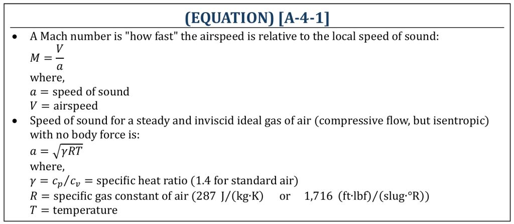
A speed of sound (a) is an important baseline unit for an airspeed measurement for an aircraft (V).  The Mach number of airspeed (M) is commonly used in aerodynamics, indicating “how fast the airspeed is” relative to the local speed of sound (a).  For an ideal gas of air, the speed of sound is commonly known as a function of local temperature of the flow field.  The equation of speed of sound is derived from the fact that a sound wave is a propagation within a non-moving atmosphere under steady and inviscid condition with no body force involved (i.e., Euler’s equation).

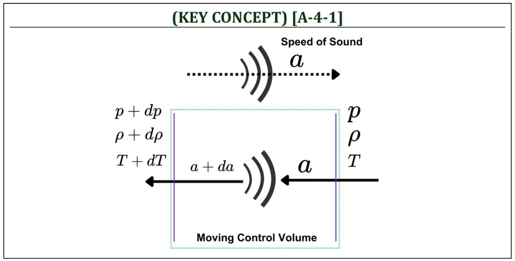
Let us take a close look at a sound wave (a weak disturbance within a non-moving flow field, that is atmosphere) generated from a source (a weak disturbance that generates a “sound”).  This sound wave will propagate with the speed of sound.  Applying Reynolds Transport theorem with a moving control volume (a control volume attached to, and thus moving the same speed with, this sound wave).  This will make it possible to analyze the system as a steady state problem.

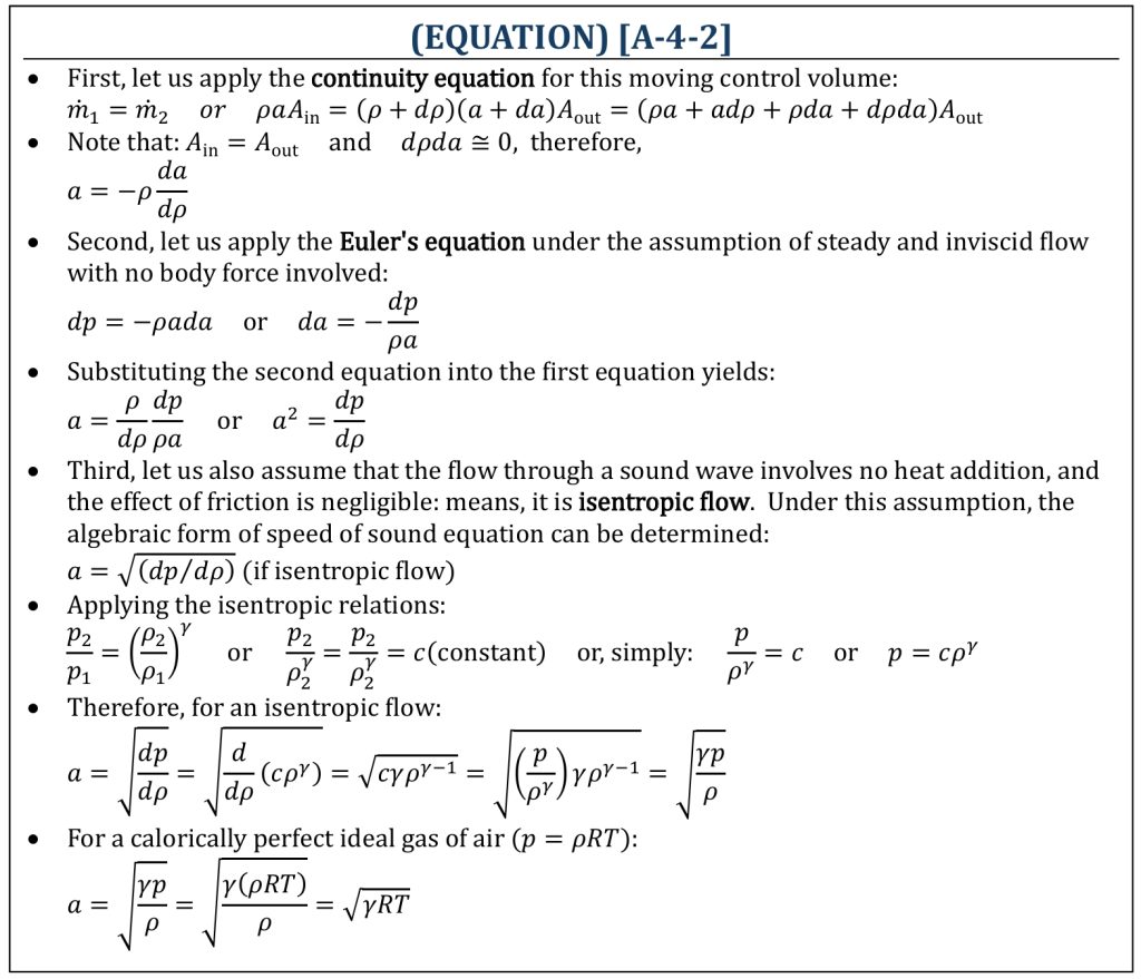
In summary, the speed of sound equation is developed by applying (i) continuity, (ii) momentum (Euler’s equation), and (iii) isentropic relations (energy is conserved) under the assumptions of steady, inviscid, no body force, and isentropic process of sound wave propagation within non-moving air (atmosphere).  Also, it is assumed calorically perfect ideal gas of air (γ = 1.4).

Pitot-Static System

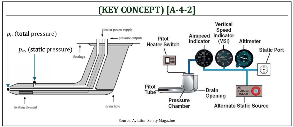
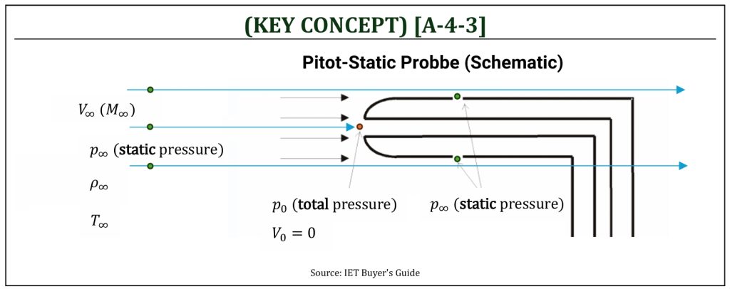
A simple airspeed indicating system can be constructed by pitot-static system for a differential pressure measurement (i.e., manometer or pressure transducer) with a simple application of Bernoulli’s equation.  Pitot-static probe measures both stagnation (or total) pressure and static pressure: provides pressure difference between them.  This is, in fact, the kinetic energy component of the air flow, called the dynamic pressure.

Let us define some important definitions first:

Static pressure (p_∞) at a given point is the pressure we would feel if we were moving along with the flow at that point.

Total pressure (p₀) at a given point in a flow is the pressure that would exist if the flow was slowed down isentropically to zero velocity (i.e., no energy loss due to friction): therefore, p_∞ < p₀ (for a stagnant air: p_∞ = p₀).

Dynamic pressure is a pressure due to the added energy into the moving fluid (air).  The difference between total and static pressures is dynamic pressure (q).  Dynamic pressure is zero for a stagnant air (p_∞ = p₀).

Stagnation point is where the airspeed becomes zero (V = 0); therefore, at stagnation point, the pressure becomes very close to the total pressure (p₀).  Especially for a low-speed aircraft, the stagnation pressure is often approximately equal to the total pressure (as the energy loss due to friction can be negligibly small: isentropic).

For an aircraft application, a differential pressure gauge is used (instead of a manometer for a wind tunnel application) to determine the dynamic pressure (q).  The static and total pressure lines are connected to opposite sides of a diaphragm.  The pressure difference causes the diaphragm to deflect.  A linkage connected to the diaphragm moves a needle on the gauge dial.  By calibrating the dial scale in terms of velocity (instead of pressure), the differential pressure gauge becomes an airspeed indicator.

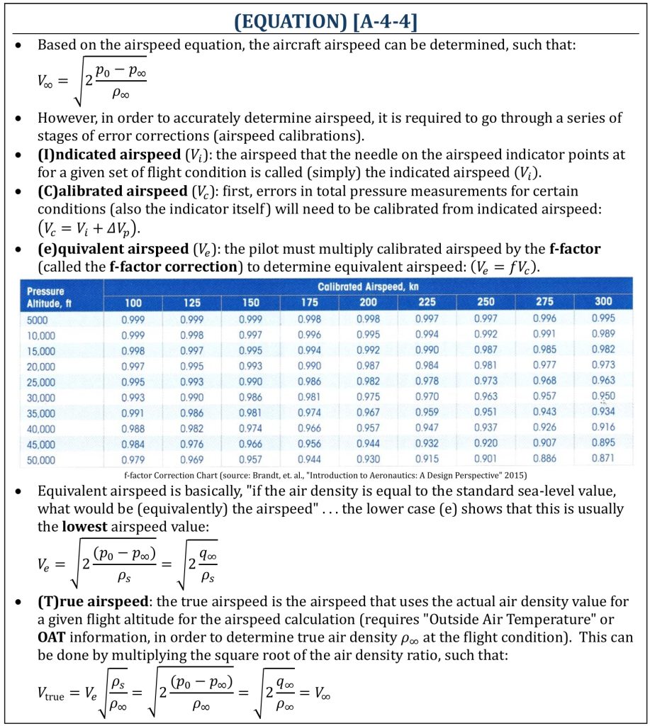
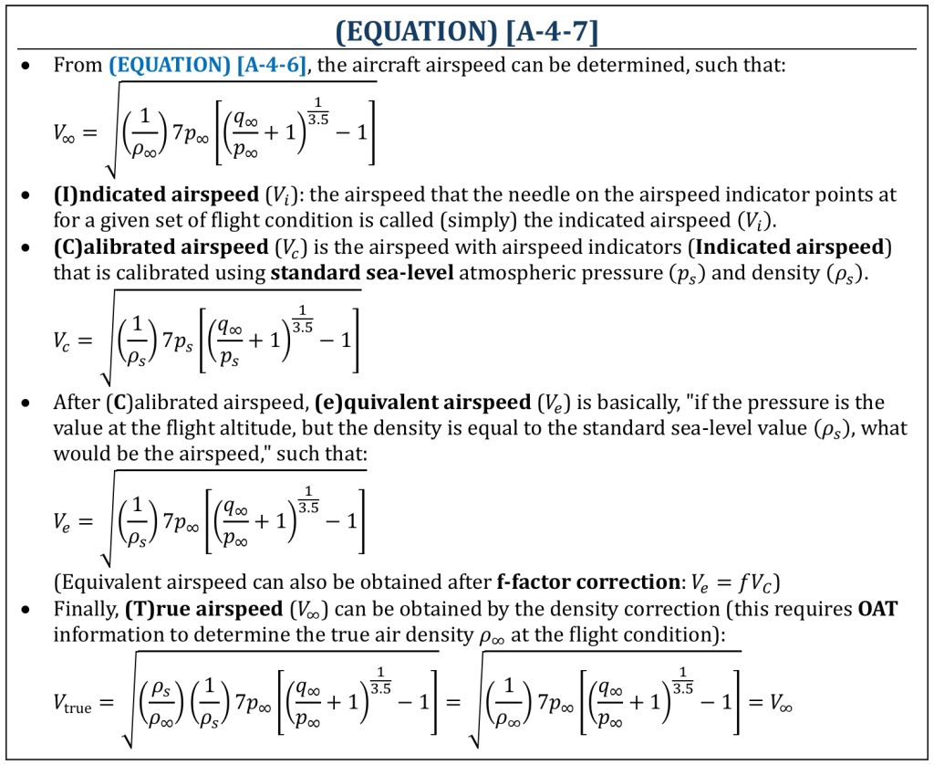
The airspeed that the needle on the airspeed indicator points at for a given set of flight condition is called (simply) the indicated airspeed (V_i).  However, usually, this indicated airspeed is NOT the speed at which the aircraft is moving through the air.  You must understand that the accurate measurement of airspeed requires a series of error corrections and calibrations.  The process can be understood as Indicated to Calibrated to Equivalent to True (ICeT).  Often also added to Ground (ICeTG) airspeed.  The lower case “e” being used as a reminder that equivalent airspeed is usually less than the other airspeeds.

Airspeed Measurement

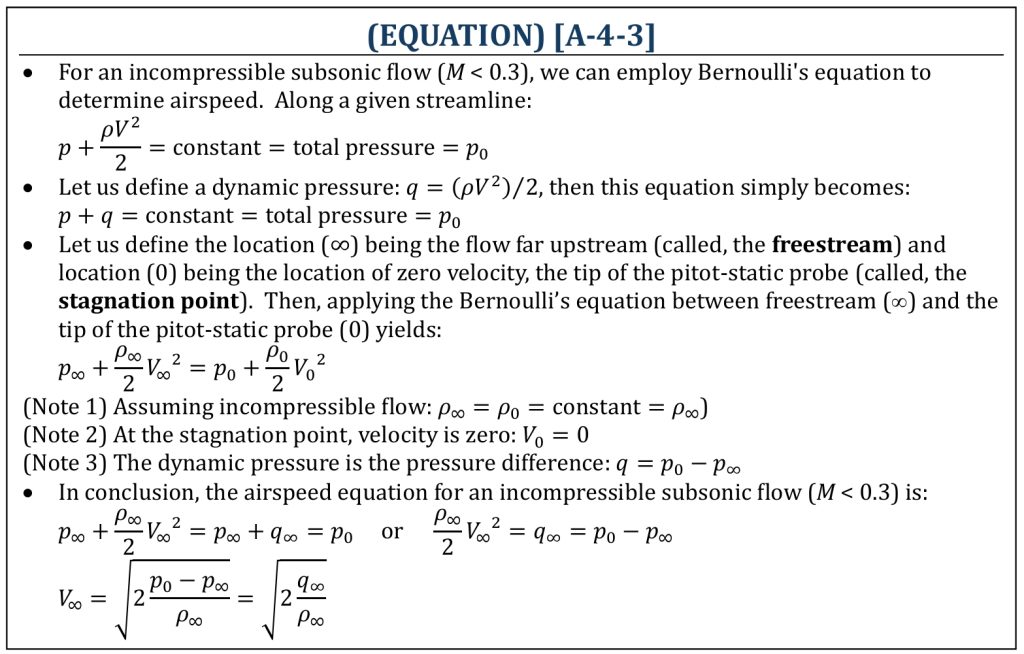
For an incompressible subsonic flow (M < 0.3), we can certainly employ Bernoulli’s equation to determine airspeed.  An important underlying concept is that the air density remains constant (ρ = constant).

Based on the airspeed equation, the aircraft airspeed can be determined.  However, in order to accurately determine airspeed from actual physical measurement, it is required to go through a series of stages of error corrections (ICeT airspeed calibrations).  A series of ICeT airspeed calibration process can be quickly done by using a simple flight computer device by a pilot during a flight of an aircraft.

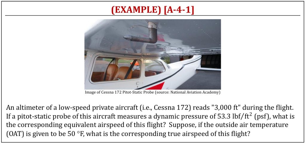
(NOTE) Airspeed in kn (knots, often also in “kts“) is a “nautical miles per hour.”  A nautical mile is based on the circumference of the earth, and is equal to one minute of latitude.  It is, in fact, slightly more than a “statute” mile (land measured: commonly used “mile”).  The unit conversion is: 1 nautical mile = 1.1508 statute miles.  Nautical miles are commonly used for charting and navigating in aeronautics/aviation (aircraft pilots).

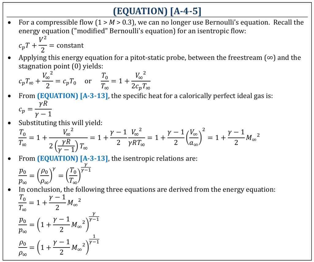
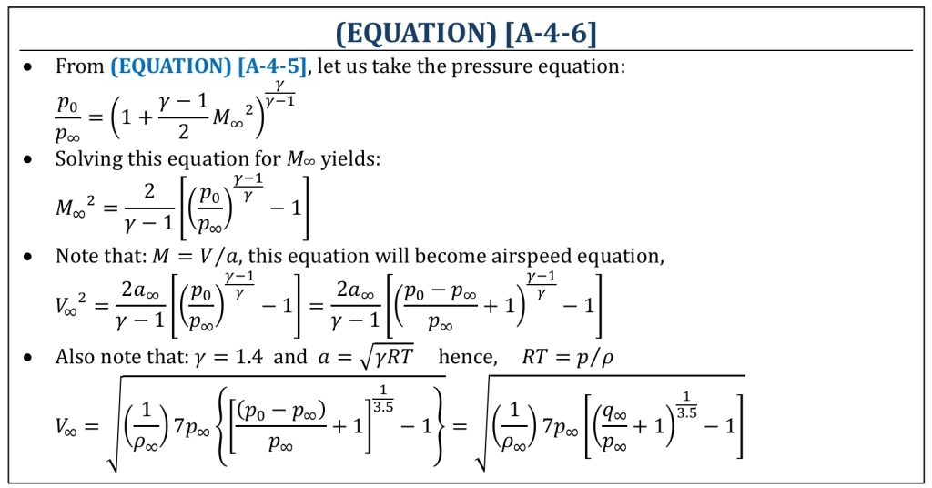
For a compressible flow (1 > M > 0.3), we can no longer use Bernoulli’s equation (the density is no longer a constant property).  Let us take a close look at the energy equation (“modified” Bernoulli’s equation for compressible flow field) one more time.

(once again) Based on the airspeed equation, the aircraft airspeed can be determined.  However, in order to accurately determine airspeed from actual physical measurement, it is required to go through a series of stages of error corrections (ICeT airspeed calibrations).  A series of ICeT airspeed calibration process can be quickly done by using a simple flight computer device by a pilot during a flight of an aircraft.

What makes the flow “incompressible” for M < 0.3 ?  So far, we employed the rule of thumb (M_∞ < 0.3) as an indicator of incompressible flow.  Let us properly understand “why” this is valid?

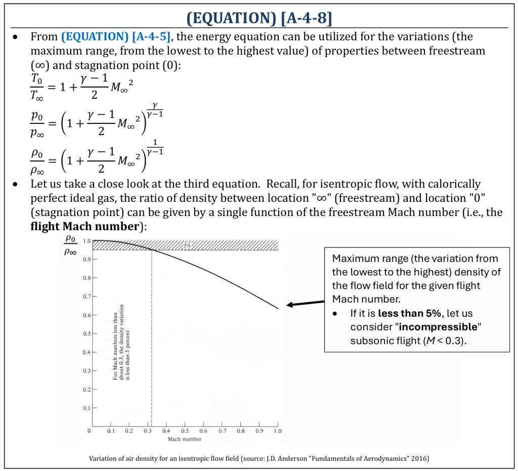
Note that the “freestream” is the location where the density is (most likely) “lowest” within the given flow field (typically, atmosphere at a flight altitude), while “stagnation point” is the location where the density is (most likely) the “highest” (most compressed).  Hence, this equation essentially represents the  maximum range of density variation within the given flow field (from lowest to highest density).  From the energy equation, this is a simple function of the freestream Mach number (M_∞).  For isentropic flows with Mach numbers less than about 0.3, the maximum density variation within the flow field is less than 5 percent.  The variation is small (insignificant), and thus the flow can be treated as incompressible.

References

• Aviation Safety Magazine (https://aviationsafetymagazine.com)
• The Institution of Engineering & Technology (https://www.theiet.org)
• The National Aviation Academy (https://www.naa.edu)
• Fundamentals of Aerodynamics by J.D. Anderson, 5th ED, McGraw Hill, 2016
• Introduction to Aeronautics: A Design Perspective by S. A. Brandt, R. J. Stiles, 3d ED, J. J. Bertin, & R. Whitford, AIAA, 2015
• Aerodynamics for Engineers by J. J. Bertin & M. L. Smith, 3rd ED, Cambridge University Press, 1997
• Aerodynamics for Engineering Students by E. L. Houghton & P. W. Carpenter, 4th ED, Edward Arnold, London, 1993

Media Attributions

If a citation and/or attribution to a media (images and/or videos) is not given, then it is originally created for this book by the author, and the media can be assumed to be under CC BY-NC 4.0 (Creative Commons Attribution-NonCommercial 4.0 International) license.  Public domain materials have been included in these attributions whenever possible.  Every reasonable effort has been made to ensure that the attributions are comprehensive, accurate, and up-to-date. The Copyright Disclaimer under Section 107 of the Copyright Act of 1976 states that allowance is made for purposes such as teaching, scholarship, and research.  Fair use is a use permitted by copyright statute.  For any request for corrections and/or updates, please contact the author.